Download
1 / 29
290 likes | 317 Vues
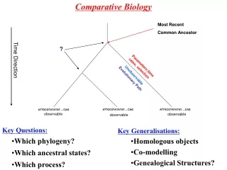
Comparative Biology. Most Recent Common Ancestor. ?. Time Direction. Parameters:time rates, selection. Unobservable Evolutionary Path. ATTGCGTATATAT….CAG. ATTGCGTATATAT….CAG. ATTGCGTATATAT….CAG. observable. observable. observable. Key Questions:. Key Generalisations:.

E N D
Comparative Biology Most Recent Common Ancestor ? Time Direction Parameters:time rates, selection UnobservableEvolutionary Path ATTGCGTATATAT….CAG ATTGCGTATATAT….CAG ATTGCGTATATAT….CAG observable observable observable Key Questions: Key Generalisations: • Which phylogeny? • Which ancestral states? • Which process? • Homologous objects • Co-modelling • Genealogical Structures?
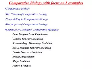
Structure of Biology: Physical Systems and Evolution Dynamics - the system as a physical entity Evolution - the system has evolved Part of individuals in a population Part of species in the tree of life • Structure of Biological Systems Framework for model formulation • Models Models M1 M1 .. Mk • Data Knowledge and Representation Scientific Texts, Systems Biology Markup Language, Process Algebras … • Knowledge & Representation Structure of Biological Systems Data Atoms, Molecules, Networks, Motors Central Dogma, Genetic Code … Sequences Structures Expression Levels …. …
The Data • Sequence Data • Expression Data • Proteomics and Protein Interactions • Metabonomics/Metabolomics and Small Molecule Detection • Structures from Crystallography, NMR and Cryo-EM • Microscopy • Single Molecule Measurements
A molecular dynamics sample path involving one catalysis event: 109 time steps 104 atoms reduction Discrete models of one catalysis event: 3-5 steps E + S ES E + P Individual molecules Set of atoms lipid molecules Concentration of molecules Nucleotide Membrane Set of E + P final states ES states? Set of E + S initial states Example of Reduction/Levels Enzyme catalysis: Such reductions can are based on “biological concepts” Other clear reductions:
Elements of Physical Dynamic Modeling 0 1 2 k Time Continuous Time No Time - Equilibrium Discrete Time State & Space p0 Complicated & contentious. Deterministic Stochastic p1 p2 p3 Continuous Time Discrete Time 0 1 k-i k-1 k Time/Space dependency Discrete Time Discrete Space Continuous Space No Space or Space Homogeneity
Physical Dynamic Modeling: Key Models Molecular Dynamics Quantum Mechanics Classical Potential Continuous Time Markov Chains/ Gillespie Algorithm Ordinary Differential Equations - ODE Partial Differential Equations - PDE (Turing Model) Stochastic Ordinary Differential Equations - SODE Stochastic Partial Differential Equations - SPDE Models on Networks Boolean Networks Kinetic Models
Elusive Biological Concepts: Emergence Other EBCs: function, robustness, modularity, purpose, top-down, downward causation. Ex.1 Network Dynamics Ex.2 Neural Networks Low dimensional “Surprising” stable, robust properties Higher level Oscillations, sensitive amplification Ability to calculate, consciousness Reduction Large set of enzymes and atoms Large set of cells High dimensional detailed description Lower level Weak emergence:something “new” emerges. Strong emergence:(never observed) The dynamic laws for k components are not deducible from their properties and their relationships. Questions:Automatic detection of emergence? How frequent is it? Does selection pull out emergent systems?
How to Compare? AGT Networks Craniums/Shape Protein Structures Homologous - Non-Homologous? Informal Homologous components A C G T A - T T Matching - Similarity - Distance Distance from shortest paths The ideal: The probability of 1 observation * Summing over possible evolutionary trajectories to the second observation. A set: A pair: P( ) P( ) ACCT ACCT Examples
“Natural” Evolutionary Modeling Discrete states: Continuous Time Finite States Markov Chains. Initially all rates the same. p0 p1 p2 p3 Continuous states: Continuous Time Continuous States Markov Process - specifically Diffusion. Initially simplest Diffusion: Brownian Motion, then Ornstein-Uhlenbeck. Components: Birth and Death Process. Components are born with rate and die with rate.
Comparative Biology Nucleotides/Amino Acids Continuous Quantities Sequences Gene Structure Structure RNA Protein Networks Metabolic Pathways Protein Interaction Regulatory Pathways Signal Transduction Macromolecular Assemblies Motors Shape Patterns Tissue/Organs/Skeleton/…. Dynamics MD movements of proteins Locomotion Culture Language Vocabulary Grammar Phonetics Semantics • Choice of Representation. • Observed or predicted?
Comparative Biology: Evolutionary Models Object Type Reference Nucleotides/Amino Acids/codons CTFS continuous time finite state Jukes-Cantor 69 +500 other Continuous Quantities CTCS Felsenstein 68 + 50 other Sequences CT countable S Thorne, Kishino Felsenstein,91 + 40 Gene Structure Matching DeGroot, 07 Genome Structure CTCS MM Structure RNA SCFG-model like Holmes, I. 06 + few others Protein Networks CT countable S Snijder, T Metabolic Pathways Protein Interaction Regulatory Pathways Signal Transduction Macromolecular Assemblies Motors I Shape Patterns Tissue/Organs/Skeleton/…. Dynamics MD movements of proteins Locomotion Culture Language Vocabulary “Infinite Allele Model” (CTCS) Swadesh,52, Sankoff,72,… Grammar - Phonetics Semantics Phenotype
“Natural” Co-Modeling • Joint evolutionary modeling of X(t),Y(t). • The ideal, rarely if ever done. • Conditional evolutionary modeling of X(t) given Y(t). The standard in comparative genomics. The distribution of Y(t) is not derived from evolution, but from practicality. • Protein Gene Prediction • RNA structure prediction • Regulatory signal prediction. • Y(t) deterministic function of X(t) • Movement of proteins • Protein Structures
Examples • RNA structure prediction • Comparative Genomics • Networks Patterns • Protein Structures
Structure Dependent Molecular Evolution RNA Secondary Structure Secondary Structure : Set of paired positions. A-U + C-G can base pair. Some other pairings can occur + triple interactions exists. Pseudoknot – non nested pairing: i < j < k < l and i-k & j-l. From Durbin et al.(1998) Biological Sequence Comparison
Simple String Generators Variables(capital)Letters(small) Regular Grammar: Start with SS --> aTbS T --> aSbT One sentence – odd # of a’s: S-> aT -> aaS –> aabS -> aabaT -> aaba Regular Context Free Context Free Grammar S--> aSabSbaa bb One sentence (even length palindromes): S--> aSa --> abSba --> abaaba
Stochastic Grammars The grammars above classify all string as belonging to the language or not. All variables has a finite set of substitution rules. Assigning probabilities to the use of each rule will assign probabilities to the strings in the language. If there is a 1-1 derivation (creation) of a string, the probability of a string can be obtained as the product probability of the applied rules. i. Start with S.S --> (0.3)aT (0.7)bS T --> (0.2)aS (0.4)bT (0.2) *0.2 *0.7 *0.3 *0.3 *0.2 S -> aT -> aaS –> aabS -> aabaT -> aaba ii. S--> (0.3)aSa (0.5)bSb (0.1)aa (0.1)bb *0.1 *0.3 *0.5 S -> aSa -> abSba -> abaaba
Secondary Structure Generators S --> LSL .869 .131 F --> dFdLS .788 .212 L --> s dFd .895 .105
From Knudsen & Hein (1999) Knudsen & Hein, 2003 RNA Structure Application
Co-Modelling and Conditional Modelling Observable Unobservable Goldman, Thorne & Jones, 96 AGGTATATAATGCG..... Pcoding{ATG-->GTG} or AGCCATTTAGTGCG..... Pnon-coding{ATG-->GTG} Knudsen.., 99 Eddy & co. C C A A Meyer and Durbin 02 Pedersen …, 03 Siepel & Haussler 03 G Pedersen, Meyer, Forsberg…, Simmonds 2004a,b • Conditional Modelling C A U U Footprinting -Signals (Blanchette) McCauley …. Firth & Brown Observable Unobservable Needs:
Network Evolution Statistics of Networks Comparing Networks Networks in Cellular Biology A. Metabolic Pathways B. Regulatory Networks C. Signaling Pathways D. Protein Interaction Networks - PIN Empirical Facts Dynamics on Networks (models) Models of Network Evolution
A given set of metabolites: • A core metabolism: Restriction R: A metabolism must define a connected graph M + R defines 1. a set of deletable (dashed) edges D(M): 2. and a set of addable edges A(M): A Model for Network Inference • A given set of possible reactions - • arrows not shown. • A set of present reactions - M • black and red arrows • Let m be the rate of deletion • l the rate of insertion • Then
Number of Metabolisms: 2 1 + 2 symmetrical versions 3 4 PQ( , )=PQ( )PQ( -> ) Approaches: Continuous Time Markov Chains with computational tricks. MCMC Importance Sampling Eleni Giannoulatou Likelihood of Homologous Pathways
A gene duplicates • Inherits it connections • The connections can change PIN Network Evolution Barabasi & Oltvai, 2004 & Berg et al. ,2004; Wiuf etal., 2006 • Berg et al. ,2004: • Gene duplication slow ~10-9/year • Connection evolution fast ~10-6/year • Observed networks can be modeled as if node number was fixed.
Irreducible (and isomorphic) 735 nodes de-DAing De-connecting Data 2386 nodes and 7221 links Likelihood of PINs Wiuf etal., 2006 • Can only handle 1 graph. • Limited Evolution Model
The Phylogenetic Turing Patterns II Spots: p large Stripes: p small Reaction-Diffusion Equations: Analysis Tasks: Choose Class of Mechanisms 2. Observe Empirical Patterns Choose Closest set of Turing Patterns T1, T2,.., Tk, Choose parameters p1, p2, .. , pk (sets?) behind T1,.. Evolutionary Modelling Tasks: 1. p(t1)-p(t2) ~ N(0, (t1-t2)S) 2. Non-overlapping intervals have independent increments I.e. Brownian Motion Scientific Motivation: Is there evolutionary information on pattern mechanisms? 2. How does patterns evolve?
Protein Structure ? ? ? ? Known Unknown Known 300 amino acid changes 800 nucleotide changes 1 structural change 1.4 Gyr a-globin Myoglobin 1. Given Structure what are the possible events that could happen? 2. What are their probabilities? Old fashioned substitution + indel process with bias. Bias: Folding(SequenceStructure) & Fitness of Structure 3. Summation over all paths.
Summary: The Virtues of Comparative Modeling P(x): C C x x A A P(Further history of x): G C A U U • It is the natural setup for much modeling and transfer of knowledge from one species/system to another. • Even 1 system/species is an evolutionary observation: