Download
1 / 68
680 likes | 727 Vues
Learn how Cellular Automata (CAs) are used to simulate various dynamic systems such as fluid dynamics, crystal growth, traffic flow, and more. Understand the algorithm and different types of CAs.

E N D
Cellular Automata This is week 7 of Biologically Inspired Computing Various credits for these slides, which have in part been adapted from slides by: Ajit Narayanan, Rod Hunt, Marek Kopicki.
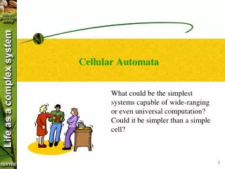
Cellular Automata • CAs have been used for simulating fluid dynamics, chemical oscillations, crystal growth, galaxy formation, stellar accretion disks, fractal patterns on mollusc shells, parallel formal language recognition, plant growth, traffic flow, urban segregation, image processing tasks, etc … • So, what are they???
Cellular Automata • A CA is a spatial lattice of N cells, each of which is one of k states at time t. • Each cell follows the same simple rule for updating its state. • The cell's state s at time t+1 depends on its own state and the states of some number of neighbouring cells at t. • For one-dimensional CAs, the neighbourhood of a cell consists of the cell itself and r neighbours on either side. Hence, k and r are the parameters of the CA. • CAs are often described as discrete dynamical systems with the capability to model various kinds ofnatural discrete or continuous dynamical systems
SIMPLE EXAMPLE Suppose we are interested in understanding how a forest fire spreads. We can do this with a CA as follows. Start by defining a 2D grid of `cells’, e.g.: This will be a spatial representation of our forest.
SIMPLE EXAMPLE continued Now we define a suitable set of states. In this case, it makes sense for a cell to be either empty, tree, or burning_tree – meaning: empty: no tree here tree: there is a tree here, and it’s healthy burning_tree: there is a tree here, and it’s on fire. When we visualise the CA, we will use colours to represent the states. In these cases; white, green and red seem the right Choices.
E.g. here ,might be an initial configuration, where the density of trees represents a particular forest we are interested in, or it may be based directly on an aerial view, and we set a randomly chosen tree to be burning.
SIMPLE EXAMPLE continued Next we define the neighbourhood structure – when we run our CA, cells will change their state under the influence of their neighbours, so we have to define what counts as a “neighbour”. You’ll see example neighbourhoods in a later slide, but usually you just use a cell’s 9 immediately surrounding neighbours. Let’s do that in this case. Next we decide what the neighbourhood will be like at the boundaries of the grid. E.g. if this was our grid, the blue are the neigbours of the green, but what are the neighbours of the red? Depending on what makes sense in the application, it could be this (fixed boundary) … … or this (wraparound)
SIMPLE EXAMPLE continued Next we define the transition rules – here we will use some simple illustrative rules – example rules for a real forest fire model appear later in the slides. For now, these are our rules – they are designed (very very roughly) to align with a timestep being one hour. R1: If a cell is empty, it’s state will stay empty at the next timestep R2: if a cell is burning, then each of its tree neighbours becomes burning at the next timestep with probability 0.2 So, starting with an initially configuration, we simply use these rules to derive a new state for every cell at each timestep.
Let’s see that in action. Here is our initial configuration, at timestep 0.
Here we are at timestep 1. I have simulated rule 2 with a random number generator somewhere in my brain.
Here we are at timestep 3. So, what will eventually happen here? What if the forest were more dense? Can you see a way to use CAs for planning new forest planting?
How a CA operates: the algorithm When a CA is set up, we decide beforehand, according to the application, what the neighbourhood is, what the wraparound situation is, what the grid dimensions are, and so on. Naturally, this includes deciding what states a cell can be in, what the transition rules are, and also we need an initial state for each cell. This is often randomised appropriately according to background knowledge (e.g. 40% trees, 60% no trees, then choose a single random tree state and set it to on_fire). SYNCHRONOUS CA then operates like this: repeat until finished: 1. for each cell: apply the rules to determine what the cell’s new state will be at the next timestep. 2. Update all cells to be in their new states An ASYNCHRONOUS CA operates like this: repeat until finished: 1. Choose a cell at random. 2. Apply the rules for that cell, and then update it to be in its new state.
Synchronous CAs Synchronous CAs can have very interesting properties, depending on the rules. Conway’s “Game of Life” is a famed very simple 2-state synchronous CA, which was formative in the establishment of a new science called Artificial Life. See the transition rules later, and the “Glider” slide (see the animation of that in Slide Show mode) From remarkably simple rules, and a very simple computational system, strange, unpredictable behaviour emerges (it is unpredictable in the sense that no theory exists which can relate the observed CA behaviour to the rules). In particular, with states and rules designed appropriately, structures which self-replicate can emerge – see the “Langton’s loops” slides.
Asynchronous CAs BOTH synchronous and asynchronous CAs are able to model natural phenomena – the HIV CA model that comes next is implemented as a synchronous CA – however asynchronous CAs would seem to be a more realistic way to model certain natural systems.
Notes on the algorithm What does “apply the rules” mean? In the CA-operation algorithm? Usually it is straightforward – e.g. suppose we have only these two rules: - if the cell is currently in state 1, and >5 neighbours are in state 0, then the cell’s new state is state 0 - in all other cases, the cell’s new state is 1 Then there is never any doubt what a cell’s next state will be, whatever the current state and the states of the neighbours. But, sometimes the rules might be under-specific, and not actually provide for a certain case. Or, they may be in conflict. This is simply something to watch out for – if you design a CA for a specific purpose, then make sure it’s operation is fully specified.
An example: a cellular automaton that models the HIV infection process in humans A fairly recent research paper (dos Santos et al) described a simple CA model of how HIV infection develops into AIDS. (find it on google scholar) There are many alternative and so-called `classical’ techniques that try to model the same process – usually this involves differential equations. However, this CA model seems to capture the quantitative dynamics of the infection more convincingly than mathematical models. This is something to do with the fact that CAs effortless combine space and time dynamics. Other techniques tend to have trouble with spatial issues, but clearly CAs are excellent at modelling processes in which the key element is neighbour interactions.
This graph is from real patient data; notice the two very different timescales on the x axis. Black is HIV-infected cells, white is healthy cells; after initial infection, HIV spreads rapidly but then subsides rapidly within weeks, after the immune system launches an initial assault which kills most of the virus. However, the virus stays around and gradually wears down the immune system in a process that can take several years. At a particular point, the density of infected cells overtakes that of healthy cells (here it is at the 8 year point); this is the onset of AIDS. Mathematical models either get the first 10 weeks correct and make a mess of the rest, or vice versa. A properly configured CA, however, can reproduce both.
dos Santos HIV CA: details A cell can be in one of 4 states: Healthy (H), Infected1 (I1), Infected2 (I2), Dead (D) There are just four rules, about what happens to a cell in the Next timestep. Rule 1 - If an H cell has at least one I1 neighbour, or if has at least 2 I2 neighbours, then it becomes I1. Otherwise, it stays healthy. Rule 2 – An I1 cell becomes I2 after 4 time steps (simulated weeks). (to operate this the CA maintains a counter associated with each I1 cell). Rule 3 - An I2 cell becomes D. Rule 4 – A D cell becomes H, with probability ; I1, with probability ; otherwise, it remains D
Notes on the HIV CA A 2D grid is used, which seems to need to be at least 400 by 400 in order to model the dynamics appropriately. Initially, a certain very small proportion of cells are randomly set to be I1. Each rule is designed based on simple but sensible notions of the biological mechanism. The probability parameters in the rules are guessed within reasonable and plausible limits based on known data. Note the counter in rule 2 – operating such a counter goes outside the `pure’ CA operation algorithms presented earlier. However, this can be simulated within the pure algorithm simply by having more states and new and different rules. (how?). But it is common practice to simplify things by using such mechanisms where appropriate. Put another way, a pure CA is computationally `complete’ – it can do anything; but in many modelling tasks it is simpler to make it impure.
Now give it a try A previous student implemented the dos Santos HIV CA in java – Find that linked from my teaching page; compile with javac *.java and the run with java Main Then choose “Run”, obviously, from the menu. Blue cells are healthy, yellow are I1 and red are I2 – each update is one week. Notice craziness (but qualitatively correct dynamics) in the first Few weeks – then, notice the onset of AIDS at around the 8 year point. If it doesn’t happen, then just try it again. Naturally you can view the code and see how the rules are Implemented. (I don’t suggest that this is exemplary java though)
Here are some well-known types of neighbourhood Many more neighbourhood techniques exist - see http://cell-auto.com and follow the link to ‘neighbourhood survey’
Classes of cellular automata (Wolfram) You recall we said that SYNCHRONOUS CAs had rather interesting properties, and were central to the research field of “Artificial Life” – these classes of CAs, defined by Steve Wolfram, are about such CAs – basically, depending on the transition rules, you tend to get one of these four types of behaviour. Class 4 is where the special things are. Class 1: after a finite number of time steps, the CA tends to achieve a unique state from nearly all possible starting conditions (limit points) Class 2: the CA creates patterns that repeat periodically or are stable (limit cycles) – probably equivalent to a regular grammar/finite state automaton Class 3: from nearly all starting conditions, the CA leads to aperiodic-chaotic patterns, where the statistical properties of these patterns are almost identical (after a sufficient period of time) to the starting patterns (self-similar fractal curves) – computes ‘irregular problems’ Class 4: after a finite number of steps, the CA usually dies, but there are a few stable (periodic) patterns possible (e.g. Game of Life) - Class 4 CA are believed to be capable of universal computation
John Conway’s Game of Life • 2D cellular automata system. • Each cell has 8 neighbors - 4 adjacent orthogonally, 4 adjacent diagonally. This is called the Moore Neighborhood.
Simple rules, executed at each time step: • A live cell with 2 or 3 live neighbors survives to the next round. • A live cell with 4 or more neighbors dies of overpopulation. • A live cell with 1 or 0 neighbors dies of isolation. • An empty cell with exactly 3 neighbors becomes a live cell in the next round.
Is it alive? • http://www.bitstorm.org/gameoflife/ • Compare it to the definitions…
Glider (animated – see this in slideshow mode) – if you happen to have the initial configuration right, this is what happens
More Sequence leading to Blinkers Clock Barber’s pole
Langton’s loops; a synchronous CA that leads to self-replicating structures 0 – Background cell state 3, 5, 6 – Phases of reproduction 1 – Core cell state 4 – Turning arm left by 90 degrees 2 – Sheath cell state state 7 – Arm extending forward cell state
There remains debate and interest about the `essentials of life’ issue with CAs, but their main BIC value is as modelling techniques. We’ve seen HIV – here are some more examples. Modelling Sharks and Fish: Predator/Prey Relationships Bill Madden, Nancy Ricca and Jonathan Rizzo Graduate Students, Computer Science Department Research Project using Department’s 20-CPU Cluster
This project modeled a predator/prey relationship • Begins with a randomly distributed population of fish, sharks, and empty cells in a 1000x2000 cell grid (2 million cells) • Initially, • 50% of the cells are occupied by fish • 25% are occupied by sharks • 25% are empty
Here’s the number 2 million • Fish: red; sharks: yellow; empty: black
Rules A dozen or so rules describe life in each cell: • birth, longevity and death of a fish or shark • breeding of fish and sharks • over- and under-population • fish/shark interaction • Important: what happens in each cell is determined only by rules that apply locally, yet which often yield long-term large-scale patterns.
Do a LOT of computation! • Apply a dozen rules to each cell • Do this for 2 million cells in the grid • Do this for 20,000 generations • Well over a trillion calculations per run! • Do this as quickly as you can
Rules in detail: Initial Conditions Initially cells contain fish, sharks or are empty • Empty cells = 0 (black pixel) • Fish = 1 (red pixel) • Sharks = –1 (yellow pixel)
Rules in detail: Breeding Rule Breeding rule: if the current cell is empty • If there are >= 4 neighbors of one species, and >= 3 of them are of breeding age, • Fish breeding age >= 2, • Shark breeding age >=3, and there are <4 of the other species: then create a species of that type • +1= baby fish (age = 1 at birth) • -1 = baby shark (age = |-1| at birth)
Rules in Detail: Fish Rules If the current cell contains a fish: • Fish live for 10 generations • If >=5 neighbors are sharks, fish dies (shark food) • If all 8 neighbors are fish, fish dies (overpopulation) • If a fish does not die, increment age
Rules in Detail: Shark Rules If the current cell contains a shark: • Sharks live for 20 generations • If >=6 neighbors are sharks and fish neighbors =0, the shark dies (starvation) • A shark has a 1/32 (.031) chance of dying due to random causes • If a shark does not die, increment age
Shark Random Death: Before I Sure Hope that the random number chosen is >.031
Shark Random Death: After YES IT IS!!! I LIVE
Results • Next several screens show behavior over a span of 10,000+ generations