CPU Scheduling

1. CPU Scheduling Objectives • Basic Concepts • Scheduling Criteria • Scheduling Algorithms • Multiple-Processor Scheduling • Real-Time Scheduling • Algorithm Evaluation

2. Basic Concepts • In multiprogramming systems, where there is more than one process runnable (ready), the OS must decide which one to run next • We already talked about the dispatcher, whose job is to allow the next process to run • It’s intimately associated with a scheduler whose job is to decide (using a scheduling algorithm) which process to have the dispatcher dispatch • We will focus on the scheduling, understand the problems associated with it, and look at some scheduling algorithms

3. Alternating Sequence of CPU And I/O Bursts

4. Nature of Processes • Not all processes have an even mix of CPU and I/O usage • A number crunching program may do a lot of computation and minimal I/O • This is an example of a CPU-BOUND process • A data processing job may do little computation and a lot of I/O • This is an example of an I/O-BOUND process

5. Types of Schedulers • We have to decide which ready process to execute next – this is Short-Term Scheduling and occurs frequently • Short-term scheduling only deals with jobs that are currently resident in memory • Jobs are constantly arriving, and Long-Term Scheduling must decide which to let into memory and in what order • Medium-Term Scheduling involves suspending or resuming processes by swapping (rolling) them out of or into memory (from disk)

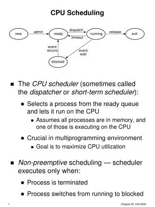
6. CPU Scheduler • Selects from among the processes in memory that are ready to execute, and allocates the CPU to one of them • CPU scheduling decisions may take place when a process: 1. Switches from running to waiting state 2. Switches from running to ready state 3. Switches from waiting to ready 4. Terminates • Scheduling under 1 and 4 is nonpreemptive • All other scheduling is preemptive

7. CPU Scheduler • Nonpreemptive scheduler means: a process is never FORCED to give up control of the CPU. The process gives up control of the CPU only • If it isn't using the CPU • If it is waiting for I/O • If it is finished using the CPU • Preemptive scheduling is forcing a process to give up control of the CPU

8. Dispatcher • Dispatcher module gives control of the CPU to the process selected by the short-term scheduler; this involves: • Switching context • Switching to user mode • Jumping to the proper location in the user program to restart that program • Dispatch latency– time it takes for the dispatcher to stop one process and start another running

9. Scheduling Criteria • The goal of CPU scheduling is to optimize system performance • But there are many factors to consider: • CPU utilization: keep the CPU as busy as possible • Throughput: # processes run per unit time • Total service time (turnaround time): time from submission to completion • Waiting Time: time spent in the ready queue • Response time: time to delivery of first result • much more useful in interactive systems

10. Additional Scheduling Criteria • There are also other elements to consider: • Priority/Importance of work – hopefully more important work can be done first • Fairness – hopefully eventually everybody is served • Implement policies to increase priority as we wait longer… (this is known as “priority aging”) • Deadlines – some processes may have hard or soft deadlines that must be met • Consistency and/or predictability may be a factor as well, especially in interactive systems

11. Optimization Criteria • Max CPU utilization • Max throughput • Min turnaround time • Min waiting time • Min response time • In other words, we want to maximize CPU utilization and throughput AND minimize turnaround, waiting, and response times

12. P1 P2 P3 0 24 27 30 First-Come, First-Served (FCFS) Scheduling ProcessBurst Time P1 24 P2 3 P3 3 • Suppose that the processes arrive in the order: P1 , P2 , P3 The Gantt Chart for the schedule is: • Waiting time for P1 = 0; P2 = 24; P3 = 27 • Average waiting time: (0 + 24 + 27)/3 = 17

13. P2 P3 P1 0 3 6 30 FCFS Scheduling (Cont.) • Suppose that the processes arrive in the order P2 , P3 , P1 • The Gantt chart for the schedule is: • Waiting time for P1 = 6;P2 = 0; P3 = 3 • Average waiting time: (6 + 0 + 3)/3 = 3 • Much better than previous case

14. Convoy Effect process service turnaround waiting time ts time tt time tw A 10 10 0 B 1 11 10 C 3 14 11 D 4 18 14 AVERAGE 13.25 8.75 process A long CPU-bound job may hog the CPU and force shorter (or I/O-bound) jobs to wait for prolonged periods. This in turn may lead to a lengthy queue of ready jobs, and hence to the 'convoy effect' A 10 B 1 C 3 D 4 time 5 10 15 20 25

15. FCFS Scheduling (Cont.) • FCFS is: • Non-preemptive • Ready queue is a FIFO queue • Jobs arriving are placed at the end of ready queue • First job in ready queue runs to completion of CPU burst • Advantages: simple, low overhead • Disadvantages: long waiting time, inappropriate for interactive systems, large fluctuations in average turnaround time are possible

16. Shortest-Job-First (SJF) Scheduling • Associate with each process the length of its next CPU burst. Use these lengths to schedule the process with the shortest time • Two schemes: • Nonpreemptive – once CPU is given to the process it cannot be preempted until the process completes its CPU burst • Preemptive – if a new process arrives with CPU burst length less than the remaining time of current executing process, preempt. This scheme is know as the Shortest-Remaining-Time-First (SRTF) • SJF is optimal – gives minimum average waiting time for a given set of processes

17. P1 P3 P2 P4 0 3 7 8 12 16 Example of Non-Preemptive SJF Process Arrival TimeBurst Time P1 0.0 7 P2 2.0 4 P3 4.0 1 P4 5.0 4 • SJF (non-preemptive) • Average waiting time = (0 + 6 + 3 + 7)/4 = 4

18. SRTF - Shortest Remaining Time First • Preemptive version of SJF • Ready queue ordered on length of time till completion (shortest first) • Arriving jobs inserted at proper position • shortest job • Runs to completion (i.e. CPU burst finishes) or • Runs until a job with a shorter remaining time arrives (i.e. placed in the ready queue)

19. P1 P2 P3 P2 P4 P1 11 16 0 2 4 5 7 Example of Preemptive SJF (i.e., SRTF) Process Arrival TimeBurst Time P1 0.0 7 P2 2.0 4 P3 4.0 1 P4 5.0 4 • Preemptive SJF (i.e., SRTF) • Average waiting time = (9 + 1 + 0 +2)/4 = 3

20. Shortest-Job-First (SJF) Scheduling • Ready queue treated as a priority queue based on smallest CPU-time requirement • Arriving jobs inserted at proper position in queue • Shortest job (1st in queue) runs to completion • In general, SJF is often used in long-term scheduling • Advantages: provably optimal w.r.t. average waiting time • Disadvantages: Unimplementable at the level of short-term CPU scheduling. Also, starvation is possible! • Can do it approximately: use exponential averaging to predict length of next CPU burst ==> pick shortest predicted burst next!

21. Determining Length of Next CPU Burst • Can only estimate the length • Can be done by using the length of previous CPU bursts, using exponential averaging a = 0 implies making no use of recent history (t n+1 = t n) a = 1 implies tn+1 = tn (past prediction not used) a = 1/2 implies weighted (older bursts get less and less weight)

22. Prediction of the Length of the Next CPU Burst This figure is for

23. Priority Scheduling • A priority number (integer) is associated with each process • Priority can be internally computed (e.g., may involve time limits, memory usage) or externally (e.g., user type, funds being paid) • In SJF, priority is simply the predicted next CPU burst time • The CPU is allocated to the process with the highest priority (smallest integer might mean highest priority) • A priority scheduling mechanism can be • Preemptive or Nonpreemptive • Starvation is a problem, where low priority processes may never execute • Solution: as time progresses, the priority of the long waiting (starved) processes is increased. This is called aging

24. 10 1 3 4 Priority Scheduling process priority service turnaround waiting time ts time tt time tw A 4 10 18 8 B 3 1 8 7 C 2 3 7 4 D 1 4 4 0 AVERAGE 9.25 4.75 process A B C D time 5 10 15 20 25

25. Round Robin (RR) • RR reduces the penalty that short jobs suffer with FCFS by preempting running jobs periodically • Each process gets a small unit of CPU time (time quantum), usually 10-100 milliseconds • The CPU blocks the current job when its reserved time quantum (time-slice) is exhausted • The current job is then put at the end of the ready queue if it has not yet completed • If the current job is completed, it will exit the system (terminate)

26. Round Robin (RR) • If there are n processes in the ready queue and the time quantum is q, then each process gets 1/n of the CPU time in chunks of at most q time units at once. No process waits more than (n -1)q time units • Performance: the critical issue with the RR policy is the length of the quantum q • q is large: RR will behave like FIFO and hence interactive processes will suffer • q is small: the CPU will be spending more time on context switching • q must be large with respect to context switch, otherwise overhead is too high

27. P1 P2 P3 P4 P1 P3 P4 P1 P3 P3 0 20 37 57 77 97 117 121 134 154 162 Example of RR with Time Quantum = 20 ProcessBurst Time P1 53 P2 17 P3 68 P4 24 • The Gantt chart is: • Typically, higher average turnaround than SJF, but better response

28. Time Quantum and Context Switch Time

29. Turnaround Time Varies With The Time Quantum • Increasing the time quantum does not necessarily improve the average turnaround time!

30. Summary of CPU Scheduling Algorithms • First-Come, First-Served (FCFS) Scheduling • Shortest-Job-First (SJF) Scheduling • Nonpreemptive • Preemptive or Shortest Remaining Time First (SRTF) • Priority Scheduling • Preemptive • Nonpreemptive • Round Robin (RR) As a practice, please solve problems 5.3, 5.4, and 5.5 on page 187 of the textbook

31. Multilevel Queue Scheduling • Ready queue is partitioned into separate queues: • For example, foreground (interactive) and background (batch) • Each queue has its own scheduling algorithm: • Foreground – RR • Background – FCFS • Scheduling must be done between the queues • Fixed priority scheduling; (i.e., serve all from foreground then from background) • Possibility of starvation • Time slice – each queue gets a certain amount of CPU time which it can schedule amongst its processes • i.e., 80% to foreground in RR and 20% to background in FCFS

32. Multilevel Queue Scheduling

33. Example of Multilevel Feedback Queue • Three queues: • Q0– time quantum 8 milliseconds • Q1– time quantum 16 milliseconds • Q2– FCFS • Scheduling • A new job enters queue Q0which is servedFCFS. When it gains CPU, the job receives 8 milliseconds. If it does not finish in 8 milliseconds, the job is moved to queue Q1 • At Q1 , the job is again served FCFS and receives 16 additional milliseconds. If it still does not complete, it is preempted and moved to queue Q2

34. Multilevel Feedback Queue

35. Multiple-Processor Scheduling • CPU scheduling is more complex when multiple CPUs are available • A multiprocessor system can have: • Homogeneous processors • Processors are identical in their functionality. Any available processor can be used to run any of the processes in the ready queue • In this class of processors, load sharing can occur • Heterogeneous processors • Processors are not identical. That is, only programs compiled for a given processor's instruction set could be run on that processor

36. Multiple-Processor Scheduling • If identical processors are available, then: • Can provide a separate ready queue for each processor • Can provide a common ready queue • Enables load sharing. All processors go into one queue and are scheduled onto any available processor • Symmetric multiprocessing: each processor is self-scheduling • We must insure that two processors do not select the same process • We must insure that processes are not lost from the ready queue • Asymmetric multiprocessing: only one processor accesses the system data structures, alleviating the need for data sharing • Master-slave relationship

37. Real-Time Scheduling • Real-time computing is divided into two types: • Hard real-time systems: required to complete a critical task within a guaranteed amount of time • Soft real-time computing: requires that critical processes receive priority over less fortunate ones • Hard real-time systems: • Resource reservation • Soft real-time systems are less restrictive • The dispatch latency must be small • The priority of real-time processes must not degrade • Disallow aging • The priority of non-real-time processes might degrade

38. Dispatch Latency • To keep the dispatch latency low • System calls have to be preemptible • But what if a high priority process needs to access data currently being modified by a lower priority process • Solution: enable priority inversion through the priority-inheritance protocol

39. Algorithm Evaluation • How do we select a CPU-scheduling algorithm for a particular system? • We must define the measures to be used in selecting the CPU scheduler and we must define the relative importance of these measures • After the selected measures have been defined, than we can evaluate the various algorithms under consideration • The different evaluation algorithms are: • Deterministic modeling • Queuing models • Simulation • Implementation

40. Algorithm Evaluation – Deterministic Modeling • One type of analytical evaluation • Deterministic modeling takes a particular predetermined workload and defines the performance of each algorithm for that workload • Deterministic modeling is • Simple and fast • Gives exact number allowing algorithms to be compared • BUT, • Requires exact input data • Its answers apply to only those input cases • In general, deterministic modeling is too specific and requires exact knowledge

41. Algorithm Evaluation – Queuing Models • Since processes running on systems vary with time, there is static set of processes to use for deterministic modeling • We can determine some parameters such as: • The distribution of the CPU burst, the distribution of the I/O burst • These distributions can be measured or estimated • For example, we have a distribution for CPU burst (service time), arrival time, waiting time, and so on • Therefore, the computer system can be described by a network of servers

42. input output server queue Algorithm Evaluation – Queuing Models • Queuing analysis can be useful in comparing the performance of scheduling algorithms • But, queuing analysis is still only an approximation of the real system • Since distributions are only estimates of the real pattern

43. Algorithm Evaluation – Simulations • Simulations give us more accuracy • Simulations involve programming a model of the computer system • The simulator has a variable representing a clock • The common way to drive the simulation is to use a random-number generator • According to a probability distribution, the random-number generator is programmed to generate processes, CPU burst times, arrivals, etc • A distribution-driven simulation may be inaccurate • The distribution indicates only how many and not the order • To resolve this problem, we can use a trace tape obtained by monitoring the real system and recording the sequence of the actual events

44. Evaluation of CPU Schedulers by Simulation

45. Algorithm Evaluation – Implementation • The only completely accurate way to evaluate a scheduling algorithm is to code it, deploy it in the OS, and see how it works • The major difficulty is the cost involved • Coding and modifying the OS • Users’ reaction • Another difficulty is that the environment in which the algorithm is used will change • Performance of the scheduler

46. Solaris 2 Scheduling

47. Windows 2000 Priorities

48. Linux Scheduling for time-sharing processes • When a new task must be chosen, the process with the most credits is selected • Every time a timer interrupt occurs, the currently running process loses one credit • When its credit reaches 0 it is suspended and another process gets a chance • If no runnable process has any credits, every process is re-credited using the formula:credits=(credits/2) + priority • This mixes the process‘s behaviour history (half its earlier credits) with its priority