CPU Scheduling
CPU Scheduling. CS 6560: Operating Systems Design. What and Why?. What is processor scheduling? Why? At first to share an expensive resource – multiprogramming Now to perform concurrent tasks because processor is so powerful Future looks like past + now

CPU Scheduling
E N D
Presentation Transcript
CPU Scheduling CS 6560: Operating Systems Design
What and Why? • What is processor scheduling? • Why? • At first to share an expensive resource – multiprogramming • Now to perform concurrent tasks because processor is so powerful • Future looks like past + now • Computing utility – large data/processing centers use multiprogramming to maximize resource utilization • Systems still powerful enough for each user to run multiple concurrent tasks
Assumptions • Pool of jobs contending for the CPU • Jobs are independent and compete for resources (this assumption is not true for all systems/scenarios) • Scheduler mediates between jobs to optimize some performance criterion • In this lecture, we will talk about processes and threads interchangeably. We will assume a single-threaded CPU.
start start idle; input idle; input idle; input idle; input stop stop Multiprogramming Example Process A 1 sec Process B Time = 10 seconds
Process A Process B start idle; input idle; input stop A start B idle; input idle; input stop B Multiprogramming Example (cont) Total Time = 20 seconds Throughput = 2 jobs in 20 seconds = 0.1 jobs/second Avg. Waiting Time = (0+10)/2 = 5 seconds
start idle; input idle; input stop A idle; input idle; input stop B Multiprogramming Example (cont) Process A context switch to B context switch to A Process B Throughput = 2 jobs in 11 seconds = 0.18 jobs/second Avg. Waiting Time = (0+1)/2 = 0.5 seconds
What Do We Optimize? • System-oriented metrics: • Processor utilization: percentage of time the processor is busy • Throughput: number of processes completed per unit of time • User-oriented metrics: • Turnaround time: interval of time between submission and termination (including any waiting time). Appropriate for batch jobs • Response time: for interactive jobs, time from the submission of a request until the response begins to be received • Deadlines: when process completion deadlines are specified, the percentage of deadlines met must be promoted
Design Space • Two dimensions • Selection function • Which of the ready jobs should be run next? • Preemption • Preemptive: currently running job may be interrupted and moved to Ready state • Non-preemptive: once a process is in Running state, it continues to execute until it terminates or blocks
Job Behavior • I/O-bound jobs • Jobs that perform lots of I/O • Tend to have short CPU bursts • CPU-bound jobs • Jobs that perform very little I/O • Tend to have very long CPU bursts CPU Disk
(Short-Term) CPU Scheduler • Selects from among the processes in memory that are ready to execute, and allocates the CPU to one of them. • CPU scheduling decisions may take place when a process: • 1. Switches from running to waiting state. • 2. Switches from running to ready state. • 3. Switches from waiting to ready. • 4. Terminates.
Dispatcher • Dispatcher module gives control of the CPU to the process selected by the short-term scheduler; this involves: • switching context • switching to user mode • jumping to the proper location in the user program to restart that program • Dispatch latency – time it takes for the dispatcher to stop one process and start another running.
P1 P2 P3 0 24 27 30 First-Come, First-Served (FCFS) Scheduling • Example: ProcessBurst Time • P1 24 • P2 3 • P3 3 • Suppose that the processes arrive in the order: P1 , P2 , P3 • The Gantt Chart for the schedule is: • Waiting time for P1 = 0; P2 = 24; P3 = 27 • Average waiting time: (0 + 24 + 27)/3 = 17
FCFS Scheduling (Cont.) • Suppose that the processes arrive in the order • P2 , P3 , P1 . • The Gantt chart for the schedule is: • Waiting time for P1 = 6;P2 = 0; P3 = 3 • Average waiting time: (6 + 0 + 3)/3 = 3 • Much better than previous case. • Convoy effect short process behind long process P2 P3 P1 0 3 6 30
Shortest-Job-First (SJF) Scheduling • Associate with each process the length of its next CPU burst. Use these lengths to schedule the process with the shortest time. • Two schemes: • Non-preemptive – once CPU given to the process it cannot be preempted until completes its CPU burst. • Preemptive – if a new process arrives with CPU burst length less than remaining time of current executing process, preempt. This scheme is know as the Shortest-Remaining-Time-First (SRTF). • SJF is optimal – gives minimum average waiting time for a given set of processes.
Example of Non-Preemptive SJF • ProcessArrival TimeBurst Time • P1 0.0 7 • P2 2.0 4 • P3 4.0 1 • P4 5.0 4 • SJF (non-preemptive) • Average waiting time = (0 + 6 + 3 + 7)/4 = 4 P1 P3 P2 P4 0 7 8 12 16
Example of Preemptive SJF • ProcessArrival TimeBurst Time • P1 0.0 7 • P2 2.0 4 • P3 4.0 1 • P4 5.0 4 • SJF (preemptive) • Average waiting time = (9 + 1 + 0 + 2)/4 = 3 P1 P2 P3 P2 P4 P1 11 16 0 2 4 5 7
Determining Length of Next CPU Burst • Can only estimate the length. • Can be done by using the length of previous CPU bursts, using exponential averaging. ( ) t = a + - a t t 1 . + n 1 n n
Examples of Exponential Averaging • = 0 • n+1 = n • Recent history does not count. • = 1 • n+1 = tn • Only the actual last CPU burst counts.
Round Robin (RR) • Each process gets a small unit of CPU time (time quantum), usually 1-50 milliseconds. After this time has elapsed, the process is preempted and added to the end of the ready queue. • If there are n processes in the ready queue and the time quantum is q, then each process gets 1/n of the CPU time in chunks of at most q time units at once. No process waits more than (n-1)q time units. • Performance • q large FIFO • q small q must be large with respect to context switch, otherwise overhead is too high.
P1 P2 P3 P4 P1 P3 P4 P1 P3 P3 Example: RR with Time Quantum = 20 • ProcessBurst Time • P1 53 • P2 17 • P3 68 • P4 24 • The Gantt chart is: • Typically, higher average turnaround than SJF, but better response time. 0 20 37 57 77 97 117 121 134 154 162
Priority Scheduling • A priority number (integer) is associated with each process • The CPU is allocated to the process with the highest priority (smallest integer highest priority). • Preemptive • Non-preemptive • SJF is a priority scheduling policy where priority is the predicted next CPU burst time. • Problem Starvation – low priority processes may never execute. • Solution Aging – as time progresses increase the priority of the process.
Multilevel Queue • Ready queue is partitioned into separate queues:foreground (interactive)background (batch) • Each queue has its own scheduling algorithm, foreground – RRbackground – FCFS • Scheduling must be done between the queues. • Fixed priority scheduling; i.e., serve all from foreground then from background. Possibility of starvation. • Time slice – each queue gets a certain amount of CPU time which it can schedule amongst its processes; e.g.,80% to foreground in RR • 20% to background in FCFS
Multilevel Feedback Queue • A process can move between the various queues; aging can be implemented this way. • Multilevel-feedback-queue scheduler defined by the following parameters: • number of queues • scheduling algorithms for each queue • method used to determine when to upgrade a process • method used to determine when to demote a process • method used to determine which queue a process will enter when that process needs service
Example of Multilevel Feedback Queue • Three queues: • Q0 – time quantum 8 milliseconds • Q1 – time quantum 16 milliseconds • Q2 – FCFS • Scheduling • A new job enters queue Q0. When it gains CPU, job receives 8 milliseconds. If it does not finish in 8 milliseconds, job is moved to queue Q1. • At Q1 job receives 16 additional milliseconds. If it still does not complete, it is preempted and moved to queue Q2. • After that, job is scheduled according to FCFS.
Traditional UNIX Scheduling Multilevel feedback queues 128 priorities possible (0-127; 0 most important) 1 Round Robin queue per priority At every scheduling event, the scheduler picks the highest priority non-empty queue and runs jobs in round-robin (note: high priority means low Q #) Scheduling events: Clock interrupt Process gives up CPU, e.g. to do I/O I/O completion Process termination
Traditional UNIX Scheduling • All processes assigned a baseline priority based on the type and current execution status: • swapper 0 • waiting for disk 20 • waiting for lock 35 • user-mode execution 50 • At scheduling events, all process priorities are adjusted based on the amount of CPU used, the current load, and how long the process has been waiting. • Most processes are not running/ready, so lots of computing shortcuts are used when computing new priorities.
UNIX Priority Calculation • Every 4 clock ticks a process priority is updated: • The utilization is incremented by 1 every clock tick during which process is running. • The NiceFactor allows some control of job priority. It can be set from –20 to 20. • Jobs using a lot of CPU increase the priority value. Interactive jobs not using much CPU will return to the baseline.
UNIX Priority Calculation • Very long running CPU-bound jobs will get “stuck” at the lowest priority, i.e. they will run infrequently. • Decay function used to weight utilization to recent CPU usage. • A process’s utilization at timetis decayed every second: • The system-wide load is the average number of runnable jobs during last 1 second é ù 2 load = * + u u NiceFactor ê ú - t ( t 1 ) + ( 2 load 1 ) ë û
UNIX Priority Decay • Assume 1 job on CPU. Load will thus be 1. Assume NiceFactor is 0. • Compute utilization at time N: • +1 second: • +2 seconds: • +N seconds: Utilization in the previous second
UNIX Priority Reset • When a process transitions from “blocked” to “ready” state, its priority is set as follows: tblocked é ù 2 load = * u u ê ú (t -1 ) t + ( 2 load 1 ) ë û where tblocked is the amount of time blocked.
Scheduling Algorithms • FIFO/FCFS is simple but leads to poor average turnaround times. Short processes are delayed by long processes that arrive before them • SJN and SRT alleviate the problem with FIFO, but require information on the length of each process. This information is not always available (though it can sometimes be approximated based on past history or user input) • RR achieves good response times, but favors CPU-bound jobs, which have longer CPU bursts • Feedback is a way of achieving good response times without information on process length, but is more complex than RR
Multiprocessor Scheduling • Several different policies: • Load sharing – an idle processor takes the first process out of the ready queue and runs it. Is this a good idea? How can it be made better? • Gang scheduling – all processes/threads of each application are scheduled together. Why is this good? Any difficulties? • Hardware partitions – applications get different parts of the machine. Any problems here?
Summary: Multiprocessor Scheduling • Load sharing: poor locality; poor synchronization behavior; simple; good processor utilization. Affinity or per processor queues can improve locality. • Gang scheduling: central control; fragmentation – unnecessary processor idle times (e.g., two applications with P/2+1 threads); good synchronization behavior; if careful, good locality • Hardware partitions: poor utilization for I/O-intensive applications; fragmentation – unnecessary processor idle times when partitions left are small; excellent locality and synchronization behavior
Network Queuing Diagrams CPU enter exit ready queue Disk 1 disk queue Disk 2 Network network queue I/O other I/O queue
Network Queuing Models • Circles are servers (resources), rectangles are queues • Jobs arrive and leave the system • Queuing theory lets us predict: avg length of queues, # jobs vs. service time • Little’s law: • Mean # jobs in system = arrival rate x mean response time • Mean # jobs in queue = arrival rate x mean waiting time • # jobs in system = # jobs in queue + # jobs being serviced • Response time = waiting + service • Waiting time = time between arrival and service • Stability condition: • Mean arrival rate < # servers x mean service rate per server
Example of Queuing Problem • A monitor on a disk server showed that the average time to satisfy an I/O request was 100 milliseconds. The I/O rate is 200 requests per second. What was the mean number of requests at the disk server?
Example of Queuing Problem • A monitor on a disk server showed that the average time to satisfy an I/O request was 100 milliseconds. The I/O rate is 200 requests per second. What was the mean number of requests at the disk server? • Mean # requests in server = arrival rate x response time = • = 200 requests/sec x 0.1 sec • = 20 • Assuming a single disk, how fast must it be for stability?
Example of Queuing Problem • A monitor on a disk server showed that the average time to satisfy an I/O request was 100 milliseconds. The I/O rate is 200 requests per second. What was the mean number of requests at the disk server? • Mean # requests in server = arrival rate x response time = • = 200 requests/sec x 0.1 sec • = 20 • Assuming a single disk, how fast must it be for stability? Service time must be lower than 0.005 secs.