Analyzing Time Complexity in Computation Theory
Learn about measuring complexity, big-O notation, asymptotic analysis, and time complexity classes in the theory of computation. Understand how to estimate running time and analyze algorithm efficiency with examples and definitions.

Analyzing Time Complexity in Computation Theory
E N D
Presentation Transcript
CSC 4170 Theory of Computation Time complexity Section 7.1
7.1.a Measuring complexity Definition 7.1 Let M be a deterministic TM that halts for every input. The running time or time complexity of M is the function f: N N, where f(n) is the maximum number of steps that M uses on any input of length n. If f(n) is the time complexity of M, we say that Mruns in time f(n), or that M is an f(n) time machine. Customarily we use n to represent the length of the input. If the time complexity of M is f(n) = n2+2, at most how many steps would M take to accept or reject the following strings? 0 10 01001
7.1.b What are the time complexities f(n) of: • 1. The fastest machine that decides {w | w starts with a 0}? • 2. The fastest machine that decides {w | w ends with a 0}? • 3. The following machine M1, deciding the language {0k1k | k0}: f(n) = 2 f(n) = n+2 M1 = “On input string w: 1. Scan across the tape and reject if a 0 is found to the right of a 1. 2. Repeat if both 0s and 1s remain on the tape: 3. Scan across the tape, crossing off a single 0 and a single 1. 4. If 0s still remain after all the 1s have been crossed off, or if 1s still remain after all the0s have been crossed off, reject. Otherwise, if neither 0s nor 1s remain on the tape, accept.” f(n) = something likean2+bn+c Here we are lazy to try to figure out the exact values of the constants a, b, c (though, apparently b=1). But are those constants really all that important once we know that n2 is involved?
7.1.c The exact running time of an algorithm often is a complex expression and depends on implementation and model details such as the number of states, the number of tape symbols, whether the “stay put” option is allowed, etc. Therefore, we usually just estimate time complexity, considering only “very large” inputs and disregarding constant factors. This sort of estimation is called asymptotic analysis. It is insensitive with respect to the above minor technical variations. Asymptotic analysis E.g., if the running time is f(n) = 6n3+2n2+20n+45 (n --- the length of input), on large n’s the first term dominates all other terms, in the sense that 2n2+20n+45 is less than n3, so that 6n3 < f(n) < 7n3. And, as we do not care about constant factors (which is something between 6 and 7), after disregarding it we are left with just n3, i.e. the highest of the orders of the terms. We express the above by using the asymptotic notation or big-O notation, writing f(n) = O(n3). Intuitively, O can be seen as a suppressed constant, and the expression f(n) = O(n3) as saying that, on large inputs, f(n)does not exceedn3 by more than some constant factor.
7.1.d N means natural numbers, R+ means positive real numbers The definitions of big-O and small-o Definition 7.2 Let f andg be functions f,g: NR+. Say that f(n) = O(g(n)) iff positive integersc and n0 exists such that for every integer nn0, f(n) cg(n). When f(n) = O(g(n)), we say that g(n) is an asymptotic upper bound for f(n). Intuition: “The complexity f(n) is the complexity g(n)”. We always have f(n)=O(f(n))
7.1.e How Big-O interacts with polynomial functions f(n) = O(g(n)) iff there are c and n0 such that, for every nn0, f(n) cg(n). f(n) = O(f(n)): pick c = n0= 3f(n) = O(f(n)): pick c = n0= 5n+10 = O(n): pick c = n0= 3n2+4n+2 = O(n2): pick c = n0= Generally, bdnd+ bd-1nd-1 + … + b2n2 + b1n + b0 = O(nd)
7.1.f How big-O interacts with logarithms f(n) = O(g(n)) iff there are c and n0 such that, for every nn0, f(n) cg(n). log8 n = O(log2n): pick c = n0= Remember that logb n = log2 n / log2 b = (1/log2 b) * log2 n log2n = O(log8n): pick c = n0= Hence, in asymptotic analysis, we can simply write log n without specifying the base. Remember that log nc = c log n Hence log nc = Since log cn = n log c and c is a constant, we have log cn = Generally, log cf(n) =
7.1.g More on big-O Big-O notation also appears in expressions such as f(n)=O(n2)+O(n). Here each occurrence of O represents a different suppressed constant. Because the O(n2) term dominates the O(n) term, we have O(n2)+O(n) = O(n2). Such bounds nc (c0) are called polynomial bounds. When O occurs in an exponent, as in f(n) = 2O(n), the same idea applies. This expression represents an upper bound of 2cn for some (suppressed) constant c. In other words, this is the bound dn for some (suppressed) constant d (d=2c). Such bounds dn, or more generally 2(n) where is a positive real number, are called exponential bounds. Sometimes you may see the expression f(n) = 2O(log n). Using the identity n=2log n and thus nc=2c log n, we see that 2O(log n) represents an upper bound of nc for some c. The expression nO(1) represents the same bound in a different way, because O(1) represents a value that is never more than a fixed constant.
7.1.j Time complexity classes Definition 7.7 Let t: NR+ be a function. We define the t-time complexity class, TIME(t(n)), to be the collection of all languages that are decidable by an O(t(n)) timeTuring machine. {w | w starts with a 0} TIME(n) ? {w | w starts with a 0} TIME(1) ? {w | w ends with a 0} TIME(n) ? {w | w ends with a 0} TIME(1) ? {0k1k | k0} TIME(n) ? {0k1k | k0} TIME(n2) ? {0k1k | k0} TIME(n log n) ? Every regular language A TIME(n) ? Linear time Constant time Square time
7.1.k M1 = “On input string w: 1. Scan across the tape and reject if a 0 is found to the right of a 1. 2. Repeat if both 0s and 1s remain on the tape: 3. Scan across the tape, crossing off a single 0 and a single 1. 4. If 0s still remain after all the 1s have been crossed off, or if 1s still remain after all the0s have been crossed off, reject. Otherwise, if neither 0s nor 1s remain on the tape, accept.” Asymptotic analysis of the time complexity of M1: • Stage 1 takes 2n (plus-minus a constant) steps, so it uses O(n) steps. Note that moving • back to the beginning is not explicitly mentioned there. The beauty of big-O is that • it allows us to suppress these details (ones that affect the number of steps only by a • constant factor). • Each scan in Stage 3 takes O(n) steps, and Stage 3 is repeated at most n/2 times. So, • Stage 2 (together with all repetitions of Stage 3) takes (n/2)O(n) = O(n2) steps. • Stage 4 takes (at most) O(n) steps. • Thus, the complexity is O(n)+O(n2)+O(n) = O(n2) What if we allowed the machine to cross out two 0s and two 1s one each pass? This would only yield improvement by a constant factor, and thus still remain O(n2).
7.1.l M2 = “On input string w: 1. Scan across the tape and reject if a 0 is found to the right of a 1. 2. Repeat if both 0s and 1s remain on the tape: 3. Scan across the tape, checking whether the total number of 0s and 1s remaining is even or odd. If it is odd, reject. 4. Scan again across the tape, crossing off every other 0 starting with the first 0, and then crossing off every other 1 starting with the first 1. 5. If no 0s and no 1s remain on the tape, accept. Otherwise reject.” An O(n log n) time machine for {0k1k | k0} • How many steps do each of the Stages 1, 3, 4 and 5 take? • How many times are Stages 3 and 4 are repeated? • What is the overall time complexity? Smart algorithms can often be much more efficient than brute force ones!
7.1.m M3 = “On input string w: 1. Scan across the tape and reject if a 0 is found to the right of a 1. 2. Scan across the 0s on tape 1 until the first 1. At the same time, copy the 0s onto tape 2. 3. Scan across the 1s on tape until the end of the input. For each 1 read on tape 1, cross off a 0 on tape 2 (moving right-to-left there). If all 0s are crossed off before all the 1s are read, reject. 4. If all the 0s have now been crossed off, accept. If any 0s remain, reject.” An O(n) time two-tape machine for {0k1k | k0} • How many steps do each of the Stages 1, 2, 3 and 4 take? • How many times are Stages 3 and 4 are repeated? • What is the overall time complexity? An important difference between computability theory and complexity theory: The former is insensitive with respect to “reasonable” variations of the underlying Computation models (variants of Turing machines), while the latter is: to what complexity class a given language belongs may depend on the choice of the model! Fortunately, however, time requirements do not differ greatly for typical deterministic models. So, if our classification system isn’t very sensitive to relatively small (such as linear vs. square) differences in complexity, the choice of deterministic model is not crucial.
7.1.n Single-tape vs. multitape machines Theorem 7.8 Let t(n) be a function, where t(n)n. Then every t(n) time multitape Turing machine has an equivalent O(t2(n)) time single-tape Turing machine. Proof Idea. Remember the proof of Theorem 3.13. It shows how to convert a multitape TM M into an equivalent single-tape TM S that simulates M. We need to analyze the time complexity of S. The simulation of each step of M takes O(k) steps in S, where k is the length of the active content of the tape of S (specifically, S makes two passes through its tape; a pass may require shifting, which still takes O(k) steps). How big can k be? Not bigger than the number of steps M takes, multiplied by the (constant) number c of tapes. That is, k ct(n)). Thus, S makes O(t(n)) passes through the active part of its tape, and each pass takes (at most) O(t(n)) steps. Hence the complexity of S is O(t(n)) O(t(n)) = O(t2(n)).
7.1.o Definition of time complexity for nondeterministic machines Definition 7.9 Let M be a nondeterministic TM that is a decider (meaning that, on every input, each branch of computation halts). The running time or time complexity of M is the function f: NN, where f(n) is the maximum number of steps that M uses on any branch of its computation on any input of length n, as shown below, with standing for a halting (accept or reject) state. Deterministic Nondeterministic f(n) … f(n) …
7.1.p Deterministic vs. nondeterministic machines Theorem 7.11 Let t(n) be a function, where t(n)n. Then every t(n) time single-tape nondeterministic TM has an equivalent 2O(t(n)) time deterministic single-tape TM. Proof Idea. One should remember the proof of Theorem 3.16. It shows how to convert a nondeterministic TM N into an equivalent deterministic TM D that simulates N by searching N’s nondeterministic computation tree. Each branch of that tree has length at most t(n), and thus constructing and searching it takes O(t(n)) steps. And the number of branches is bO(t(n)), where b is the maximum number of legal choices given by N’s transition function. But b2c for some constant c. So, the number of branches is in fact 2cO(t(n))=2O(t(n)). Thus, the overall number of steps is O(t(n)) 2O(t(n)) = 2O(t(n)).