Interarea Oscillations
Interarea Oscillations. Starrett Mini-Lecture #5. Interarea Oscillations - Linear or Nonlinear?. Mostly studied as a linear phenomenon More evidence of nonlinear or stressed system problem. Why do We Like Linear Systems?. Easy to solve differential equations

Interarea Oscillations
E N D
Presentation Transcript
Interarea Oscillations Starrett Mini-Lecture #5
Interarea Oscillations - Linear or Nonlinear? • Mostly studied as a linear phenomenon • More evidence of nonlinear or stressed system problem
Why do We Like Linear Systems? • Easy to solve differential equations • Can calculate frequencies and damping • Design control systems easily • Pretty good approximation
Small-Signal Stability -> Linear System Analysis • State Space representationDx = A Dx + B DuDy = C Dx + D Du • A = ¶f1/¶x1 ... ¶f1/¶xn B = {¶f/¶u}¶f2/¶x1 ... ¶f2/¶xn ...¶fn/¶x1 ... ¶fn/¶xn
Linear System Terms • Eigenvalues • Eigenvectors • Jordan Canonical Form • System Trajectories • Measures of system performance
Eigenvalues • Roots of characteristic equation • Tell stability properties of linear system (Hartman-Grobman Theorem) • Eigenvalues => l = s + jw
Linear System Solution • x(t) = C1 el1t + C2 el2t ... + Cn elnt • x(t) = C1 e(s1+ jw1)t + C2 e(s2+ jw2)t … + Cn e(sn+ jwn)t • x(t) = D1 es1tcos(w1t) + D2 es2tcos(w2t) … • Constants are dependent on initial conditions
Calculating Eigenvalues • A ri = li ri • A = system plant matrix • l = eigenvalue • r = an nX1 vector (right eigenvector) • Rearranging … • (A - lI)r = 0 => det(A - lI) = 0
Solving for Right Eigenvectors • A ri = li ri • Solve system of linear algebraic equations for components of ri, (r1i, r2i, r3i, etc.) • Right Modal Matrix, • R = square matrix with ri's as columns
Left Modal Matrix & Left Eigenvectors • L = R-1 • left eigenvectors = li's = rows of L • li A = li li
Free Response of a System of Linear Differential Equations • Dx = A Dx • Define a variable transformation • Dx = R z • Substitute into diff. eq. • R z’ = A R z • Pre-multiply both sides by R-1 = L • L R z’ = R-1R z = R-1A R z = L A R z = L z
Jordan Canonical Form • z’ = L z • L = diagonalized matrix with li's on diagonalL = l1 0 0 0 ... 0 l2 0 0 ... 0 0 l3 0 ... ... 0 0 0 ... ln
The Jordan Form System is Decoupled • z1 = l1 z1 => z1(t) = z1o el1t • z2 = l2 z2 => z2(t) = z2o el2t … • zn = ln zn => zn(t) = zno elnt
Now Transform Solutions Back to x-Space • Dx = R z => Dx(t) = R z(t) • Dx1(t) = r11 z1(t) + r12 z2(t) + ... R1n zn(t) • Dx1(t) = r11 z1oel2t + r12 z2oel2t… + r1n zno elnt
Initial Conditions • zio's are the initial conditions in z-space • xo is the vector of initial conditions in x-spaceDx = Rz => LDx = L R z => LDx = z • so . . . zo = L xo and zio = l11 x1o + l12 x2o + . . . + l1n xno
Visualize the Linear Systems Analysis x1 z1 z2 x2 Angle-Speed Space Jordan State Space
In-Class Exercise A = 1 2 3 1 1. Eigenvalues = ? 2. What values of x1o and x2o correspond to z1o = 1, z2o = 0? R = 0.6325 -0.6325 0.7746 0.7746 L = 0.7906 0.6455 -0.7906 0.6455
Answers 1 - l 2 3 1 - l
More Answers 0.6325 -0.6325 0.7746 0.7746 1 0