Download
1 / 18
180 likes | 341 Vues
Today’s Announcements. Today’s take-home lessons (i.e. what you should be able to answer at end of lecture). Homework assigned #6 (assigned last Friday; due Monday, 4/12 in class. This Wednesday: in class quiz on “take-home messages” : won’t be solely fill in the blanks.

E N D
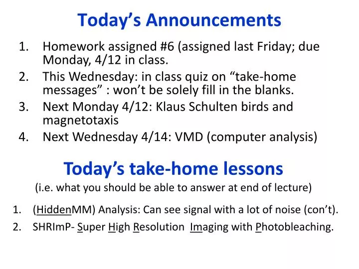
Today’s Announcements Today’s take-home lessons(i.e. what you should be able to answer at end of lecture) • Homework assigned #6 (assigned last Friday; due Monday, 4/12 in class. • This Wednesday: in class quiz on “take-home messages” : won’t be solely fill in the blanks. • Next Monday 4/12: Klaus Schulten birds and magnetotaxis • Next Wednesday 4/14: VMD (computer analysis) • (HiddenMM) Analysis: Can see signal with a lot of noise (con’t). • SHRImP- Super High Resolution Imaging with Photobleaching.
What is Hidden Markov Method (HMM)? Hidden Markov Methods (HMM) –powerful statistical data analysis methods initially developed for single ion channel recordings – but recently extended to FRET on DNA, to analyze motor protein steps sizes – particularly in noisy traces. What is a Markov method? the transition rates between the states are independent of time. Why is it called Hidden? Often times states have the same current, and hence are hidden. Also, can be “lost” in noise. What is it good for? Can derive signals where it appears to be only noise!
C O → ← Simple model (non-HMM) applied to ion channels Transitions between one or more closed states to one or more open states. (From Venkataramanan et al, IEEE Trans., 1998 Part 1.) Model (middle) of a single closed (C) and open (O) state, leading to 2 pA or 0 pA of current (middle, top), and a histogram analysis of open (left) and closed (right) lifetimes, with single exponential lifetimes. In both cases, a single exponential indicates that there is only one open and one closed state. Hence the simple model C O is sufficient to describe this particular ion channel. In general, N exponentials indicate N open (or closed) states. Hence the number of open (closed) states can be determined, even if they have the same conductance. In addition, the relative free energies of the open vs. closed two states can be determined because the equilibrium constant is just the ratio of open to closed times and equals exp(-DG/kT).
Outline con’t: Making a Markov Process Two general points: Notice that correlations between states are inherent in the topology and rate constants. (For example, if state B can only be reached through State A, then the presence of state B would indicate that state A should be found in some time before State B.) Furthermore, like the histogram method mentioned, multiple states (conformations) with the same signal (e.g. multiple open states with the same ionic conductance, or multiple closed states) can be detected via statistical analysis from their lifetime distributions.
c. a. b. Hidden Markov Models An impressive feature of combining Hidden Markov & Maximum Likelihood models is the ability to extract signal from noise. Indeed, they are often called Hidden Markov Methods because the observable (ionic current, or position in the case of molecular motors) is often hidden in the noise. Use of Hidden Markov Methods to analyze single ion channel recordings. a) Ideal current vs. time, showing ion channel transitions with two different conductivities and forward and backward rate constants of 0.3 and 0.1. B) Data of (a) added to white noise such that noise level = signal level. C) Extraction of kinetic parameters using HMM from noisy data in b, showing kinetic constants can be recovered. (Venkataramanan et al., IEEE Transactions, 1998, Part I.)
Multiple algorithms for finding best pathways. There are multiple ways to do HMM. The Viterbi algorithm is what QuB uses to idealize the data (IDL command) but Viterbi is not a guaranteed global optimum since it is a selected pathway through the data, but its much faster than the alternative, the point likelihood. The alternative is to do the maximum point likelihood (MPL command) that optimizes the parameters (amplitude and rates) over the selected data.
Molecular motors can be modeled like ion channels Conceptually a transition between a closed and open state in an ion channel corresponds to a molecular motor taking a step. A transition between one closed ion channel state and another closed state corresponds to a conformational change within the motor that does not lead to a step – e.g. hydrolysis of ATP into ADP + Pi in kinesin. These states can potentially be detected because they affect the kinetics (stepping rate and /or distribution). Hence, an important aspect of this analysis is that we may be able to discover the presence of new conformational states, likely associated with nucleotide states. In addition, if motors walk in a hand-over-hand mechanism, and there is an asymmetry between the two heads – e.g. a step where “left foot” goes forward, vs. “right foot” goes forward – and one tends to overwinds the coiled-coiled stalk, and the other tends to underwind the stalk, then this may show up in the stepping kinetics. This is analogous to an ion channel with multiple states of equal conductance.
Two kinesins operate simultaneously in vivo Must use Hidden Markov Method to see Syed, unpublished Unlikely due to microtubule motion because fairly sharply spiked around ±4-5 nm Two kinesins (+2 Dyneins), in vivo, are moving melanosome
PALM Comparative TIRF and PALM images TIRF image Magnified PALM image Vinculin-tagged dEosFP
Photo-active GFP G. H. Patterson et al., Science 297, 1873 -1877 (2002) Photoactivatable variant of GFP that, after intense irradiation with 413-nanometer light, increases fluorescence 100 times when excited by 488-nanometer light and remains stable for days under aerobic conditions Native= filled circle Photoactivated= Open squares T203H GFP: PA-GFP Wild-type GFP
Photoactivation and imaging in vitro G. H. Patterson et al., Science 297, 1873 (2002)
Can we achieve nanometer resolution? i.e. resolve two point objects separated by d << l/2? P1 P2 Breaking the Rayleigh criteria: 1st method SHRIMP Super High Resolution IMaging with Photobleaching
SHRImP on DNA (Super-High Resolution Imaging with Photobleaching)
- = Utilizing Photobleaching for Colocalization Additional knowledge: 2 single dyes When one dies, fit remaining PSF accurately; then go back and refit first PSF. Separation = 324.6 ± 1.6 nm Separation = 329.7 ± 2.2 nm
Sample Measured Distance 51-mer 17.7 ± 0.7 nm 13.0 ± 0.5 nm 40-mer 30-mer 10.7 ± 1.0 nm Control: DNA Molecule End-to-End Separation Conventional resolution: 300 nm Unconventional resolution: few nm! • DNA labeled Cy3 on 5’ end, hydridized. • Flowed over coverslip coated with nitrocellulose to prevent adverse • photophysical interaction of dye with glass • DNA binds non-specifically to NC surface • *DNA is stretched by fluid flow to 150% extension (Bensimon, Science, 1994). Gordon et al. PNAS, 2003
DNA Replication: made with very high fidelity Is each mutation independent of the another mutation? How does mutation rate depend on time?
Assume mutations accrue at constant ratei.e. probability of mutation a time. If each mutation is independent, then probability of: 2 mutations = t2 3 mutations = . . 6 mutations = t3 t6 Since Probability (cancer) ~ t6, likely that cancer caused by average of six mutations Note: This assumes that you get 6 mutations “all of a sudden,” that is, within a certain period of time, that gives you cancer. For example: If you get a mutation with a rate of 1/year, then after 2 years you have 2 mutations, after 3 years you have 3 mutations , etc. But if the body cleans up the mutation (within the time it takes you to get 6 mutations—in this case, 6 years), these don’t likely cause cancer. It’s only if you “all of a sudden” get the 6 mutations, that it causes cancer. In this case the rate at which the body “cleans up” the mutation is important.
Class evaluation 1. What was the most interesting thing you learned in class today? 2. What are you confused about? 3. Related to today’s subject, what would you like to know more about? 4. Any helpful comments. Answer, and turn in at the end of class.