Download

1 / 27
280 likes | 512 Vues
Clustering with k-means and mixture of Gaussian densities. Jakob Verbeek December 3, 2010 Course website: http://lear.inrialpes.fr/~verbeek/MLCR.10.11.php. Plan for the course. Session 1, October 1 2010 Cordelia Schmid: Introduction Jakob Verbeek: Introduction Machine Learning

E N D
Clustering with k-means and mixture of Gaussian densities Jakob Verbeek December 3, 2010 Course website: http://lear.inrialpes.fr/~verbeek/MLCR.10.11.php
Plan for the course • Session 1, October 1 2010 • Cordelia Schmid: Introduction • Jakob Verbeek: Introduction Machine Learning • Session 2, December 3 2010 • Jakob Verbeek: Clustering with k-means, mixture of Gaussians • Cordelia Schmid: Local invariant features • Student presentation 1: Scale and affine invariant interest point detectors, Mikolajczyk, Schmid, IJCV 2004. • Session 3, December 10 2010 • Cordelia Schmid: Instance-level recognition: efficient search • Student presentation 2: Scalable Recognition with a Vocabulary Tree, Nister and Stewenius, CVPR 2006.
Plan for the course • Session 4, December 17 2010 • Jakob Verbeek: Mixture of Gaussians, EM algorithm, Fisher Vector image representation • Cordelia Schmid: Bag-of-features models for category-level classification • Student presentation 2: Beyond bags of features: spatial pyramid matching for recognizing natural scene categories, Lazebnik, Schmid and Ponce, CVPR 2006. • Session 5, January 7 2011 • Jakob Verbeek: Classification 1: generative and non-parameteric methods • Student presentation 4: Large-Scale Image Retrieval with Compressed Fisher Vectors, Perronnin, Liu, Sanchez and Poirier, CVPR 2010. • Cordelia Schmid: Category level localization: Sliding window and shape model • Student presentation 5: Object Detection with Discriminatively Trained Part Based Models, Felzenszwalb, Girshick, McAllester and Ramanan, PAMI 2010. • Session 6, January 14 2011 • Jakob Verbeek: Classification 2: discriminative models • Student presentation 6: TagProp: Discriminative metric learning in nearest neighbor models for image auto-annotation, Guillaumin, Mensink, Verbeek and Schmid, ICCV 2009. • Student presentation 7: IM2GPS: estimating geographic information from a single image, Hays and Efros, CVPR 2008.
Clustering • Finding a group structure in the data • Data in one cluster similar to each other • Data in different clusters dissimilar • Map each data point to a discrete cluster index • “flat” methods find k groups (k known, or automatically set) • “hierarchical” methods define a tree structure over the data
Hierarchical Clustering Data set is partitioned into a tree structure Top-down construction Start all data in one cluster: root node Apply “flat” clustering into k groups Recursively cluster the data in each group Bottom-up construction Start with all points in separate cluster Recursively merge “closest” clusters Distance between clusters A and B Min, max, or mean distance between x in A, and y in B
Clustering example [Guillaumin, Verbeek, Schmid, ICCV 2009] Learn face similarity from training pairs labeled as same/different Cluster faces based on identity Example: picasa web albums, label face clusters
Clustering for visual vocabulary construction Clustering of local image descriptors Most often done using k-means or mixture of Gaussians Divide space of region descriptors in a collection of non-overlapping cells Recap of the image representation pipe-line Extract image regions at different locations and scales: randomly, on a regular grid, or using interest point detector Compute descriptor for each region (eg SIFT) Assign each descriptor to a cluster center Or do “soft assignment” or “multiple assignment” Make histogram for complete image Possibly separate histograms for different image regions
Definition of k-means clustering Given: data set of N points xn, n=1,…,N Goal: find K cluster centers mk, k=1,…,K Clustering: assignment of data points to cluster centers Binary indicator variables rnk =1 if xn assgined to xn, 0 otherwise Error criterion: sum of squared distances between each data point and assigned cluster center
Examples of k-means clustering Data uniformly sampled in unit square, running k-means with 5, 10, 15, 20 and 25 centers
Minimizing the error function Goal find centers mk and assignments rnk to minimize the error function An iterative algorithm Initialize cluster centers, somehow Update assignments rnk for fixed mk Update centers mk for fixed data assignments rnk fixed If cluster centers changed: return to step 2) Return cluster centers Iterations monotonically decrease error function
Examples of k-means clustering Several iterations with two centers Error function
Minimizing the error function Update assignments rnk for fixed mk Decouples over the data points Only one rnk =1, rest zero Assign to closest center Update centers mk for fixed assignments rnk Decouples over the centers Set derivative to zero Put center at mean of assigned data points
Minimizing the error function Goal find centers mk and assignments rnk to minimize the error function An iterative algorithm Initialize cluster centers, somehow Update assignments rnk for fixed mk Update centers mk for fixed data assignments rnk fixed If cluster centers changed: return to step 2) Return cluster centers Iterations monotonically decrease error function Both steps reduce the error function Only a finite number of possible assignments
Examples of k-means clustering Several iterations with two centers Error function
Examples of k-means clustering Solutions for different initializations
Examples of k-means clustering Clustering RGB vectors of pixels in images Compression of image file: N x 3 x 8 bits Store RGB values of cluster centers: K x 24 bits Store cluster index of each pixel: N x log K bits 8.3% 16.7% 4.2%
Clustering with Gaussian mixture density Each cluster represented by Gaussian density Center, as in k-means Covariance matrix: cluster spread around center Determinant of covariance matrix C Data dimension d Quadratic function of point x and mean m
Clustering with Gaussian mixture density Mixture density is weighted sum of Gaussians Mixing weight: importance of each cluster Density has to integrate to 1, so we require
Clustering with Gaussian mixture density Given: data set of N points xn, n=1,…,N Find mixture of Gaussians (MoG) that best explains data Assigns maximum likelihood to the data Assume data points are drawn independently from MoG Maximize log-likelihood of fixed data set X w.r.t. parameters of MoG As with k-means objective function has local minima Can use Expectation-Maximization (EM) algorithm Similar to the iterative k-means algorithm
Assignment of data points to clusters As with k-means zn indicates cluster index for xn To sample point from MoG Select cluster index k with probability given by mixing weight Sample point from the k-th Gaussian MoG recovered if we marginalize of unknown index
Soft assignment of data points to clusters Given data point xn, infer value of zn Conditional probability of zn given xn
Maximum likelihood estimation of Gaussian Given data points xn, n=1,…,N Find Gaussian that maximizes data log-likelihood Set derivative of data log-likelihood w.r.t. parameters to zero Parameters set as data covariance and mean
Maximum likelihood estimation of MoG Use EM algorithm Initialize MoG: parameters or soft-assign E-step: soft assign of data points to clusters M-step: update the cluster parameters Repeat EM steps, terminate if converged Convergence of parameters or assignments E-step: compute posterior on z given x: M-step: update Gaussians from data points weighted by posterior
Maximum likelihood estimation of MoG Example of several EM iterations
Clustering with k-means and MoG Hard assignment in k-means is not robust near border of quantization cells Soft assignment in MoG accounts for ambiguity in the assignment Both algorithms sensitive for initialization Run from several initializations Keep best result Nr of clusters need to be set Both algorithm can be generalized to other types of distances or densities Images from [Gemert et al, IEEE TPAMI, 2010]
Further reading material • Paper by Radford Neal & Geoffrey Hinton “A view of the EM algorithm that justifies incremental, sparse, and other variants” in “Learning in graphical models”,1998. (available online) • Chapter 9 from the book “Machine Learning and Pattern Recognition”, by Chris Bishop (Springer, 2006)