An Introduction to Binomial Trees Chapter 11
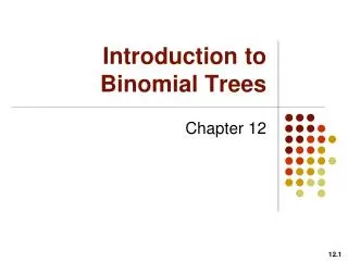
An Introduction to Binomial Trees Chapter 11. A Simple Binomial Model. A stock price is currently $20 In three months it will be either $22 or $18. Stock Price = $22. Stock price = $20. Stock Price = $18. A Call Option. A 3-month call option on the stock has a strike price of 21.

An Introduction to Binomial Trees Chapter 11
E N D
Presentation Transcript
A Simple Binomial Model • A stock price is currently $20 • In three months it will be either $22 or $18 Stock Price = $22 Stock price = $20 Stock Price = $18
A Call Option A 3-month call option on the stock has a strike price of 21. Figure 11.1 Stock Price = $22 Option Price = $1 Stock price = $20 Option Price=? Stock Price = $18 Option Price = $0
22– 1x1 18 Setting Up a Riskless Portfolio • Consider the Portfolio: long shares short 1 call option • Portfolio is riskless when 22– 1 = 18 or = 0.25
Valuing the Portfolio( Risk-Free Rate is 12% ) • The riskless portfolio is: long 0.25 shares short 1 call option • The value of the portfolio in 3 months is 220.25 – 1 = 4.50 • The value of the portfolio today is 4.5e – 0.120.25 = 4.3670
Valuing the Option • The portfolio that is long 0.25 shares short 1 option is worth 4.367 • The value of the shares is 5.000 (= 0.2520 ) • The value of the option is therefore 0.633 (= 5.000 – 4.367 )
Su ƒu S ƒ Sd ƒd Generalization • Stock goes up by u-1 percent or down by d-1 percent. • Figure 11.2
Generalization(continued) • Consider the portfolio that is long shares and short 1 derivative • The portfolio is riskless when Su– ƒu = Sd– ƒd or Su– ƒu Sd – ƒd
Generalization(continued) • Value of the portfolio at time T is Su– ƒu • Value of the portfolio today is (Su– ƒu )e–rT • Another expression for the portfolio value today is S– ƒ • Hence ƒ = S– (Su– ƒu)e–rT
Generalization(continued) • Substituting for we obtain ƒ = [ p ƒu + (1 – p )ƒd ]e–rT Eqn (11.2) p. 246 where • p is called the risk neutral probability • Hull also uses p as the put price
Generalization – Continued • Note: u > 1 and d < 1 • Note: d < erT < u (why?) • So 0 < p < 1 • Expected stock return using p equals risk-free rate
Su ƒu p S ƒ Sd ƒd (1– p ) Risk-Neutral Valuation • ƒ = [ p ƒu + (1– p )ƒd ]e-rT Eqn (11.2) • The variables p & (1– p ) can be interpreted as the risk-neutral probabilities of up and down movements • The value of a derivative is its expected payoff in a risk-neutral world discounted at the risk-free rate
Risk-Neutral Valuation • In risk-neutral world (RNW) the expected return on all assets equal the risk-free rate • Determine risk-neutral probabilities: p and 1-p • Then c = e-rT E[max{0, S-X}] = e-rT [p(S-X) + (1-p)(0)], where expectation is wrt to risk- neutral probabilities
Risk Neutral Valuation • Suppose u = 1.1, d = .95, and erT = 1.05 • Let S = $1 (it does not matter). Then in RNW E[ST] = S erT: 1.1p + .95(1-p) = 1.05 • Or p = (1.05 - .95)/(1.1 - .95) = 2/3 same as eq (10.3) • Suppose X = 100, S = 100, and payoff = max{0, ST – 100} • Then c = [(2/3)(110-100) + (1/3)(0)](1/1.05) = $6.35
Risk Neutral Valuation: Basic Idea • Option value based upon absence of arbitrage profit • Arbitrage profit desirable regardless of investors’ risk preferences • All investors regardless of risk preferences assign same value to options • So in a world of risk neutral investors options would have the same value as in risk-averse world • Equal to the present value of expected payoff
Irrelevance of Stock’s Expected Return When we are valuing an option in terms of the underlying stock the expected return on the stock is irrelevant Why? Because in a risk-neutral world options have the same value as in our risk-averse world. But all assets have an expected return equal to the risk free rate. So expected return does not matter.
Interesting Question • Suppose stock A has an expected return of 10% and a risk of 20% • Stock B has an expected return of 15% and a risk of 20% • How can the call option values be the same? • Wouldn’t you rather own option on stock B? • In a risk-neutral world both would have an expected return equal to the risk-free rate and a risk of 20%. • Therefore, both would have the same value.
Original Example Revisited Su = 22 ƒu = 1 p • Since p is a risk-neutral probability 20e0.12 0.25 = 22p + 18(1– p ); p = 0.6523 • Alternatively, we can use the formula: S ƒ Sd = 18 ƒd = 0 (1– p )
Su = 22 ƒu = 1 0.6523 S ƒ Sd = 18 ƒd = 0 0.3477 Valuing the Call Option The value of the option is e–0.120.25 [0.65231 + 0.34770] = 0.633
Su = 22 ƒu = 0 0.6523 S ƒ Sd = 18 ƒd = 3 0.3477 Valuing a Put Option struck at 21:RNVR Put option The value of the option is e–0.120.25 [0.65230 + 0.34773] = 1.0124
Su = 22 ƒu = 0 0.6523 S ƒ Sd = 18 ƒd = 3 0.3477 Valuing a Put Option: Put-Call Parity The value of the put option p = c + Xe-rT – S = .633 + 21 .97045 - 20 = 1.0124
Valuing a Put Option: Delta-Neutral Hedge • = (0 – 3)/(22 – 18) = -.75 • buy .75 shares of stock • buy 1 put • FVup = .75 22 + 0 = 16.5 • FVdown = .75 18 + 3 = 16.5 • PV = 16.5 .97045 = 16.0124 • so 16.0124 = .75 20 + p • therefore, p = 16.0124 - .75 20 = 1.0124
Delta • Delta () is the ratio of the change in the price of a stock option to the change in the price of the underlying stock • The value of varies from node to node
Delta Option price Slope = D B Stock price A • Delta (D) is the rate of change of the option price with respect to the underlying
Properties of Call Delta • Delta is positive • Increases with the underlying stock price • As S approaches 0 Delta approaches 0 • As S becomes large Delta approaches 1