Lecture 6 – Binomial trees
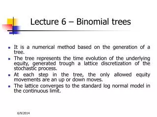
Lecture 6 – Binomial trees. It is a numerical method based on the generation of a tree. The tree represents the time evolution of the underlying equity, generated trough a lattice discretization of the stochastic process.

Lecture 6 – Binomial trees
E N D
Presentation Transcript
Lecture 6 – Binomial trees • It is a numerical method based on the generation of a tree. • The tree represents the time evolution of the underlying equity, generated trough a lattice discretization of the stochastic process. • At each step in the tree, the only allowed equity movements are an up or down moves. • The lattice converges to the standard log normal model in the continuous limit.
Binomial trees Option valuation with binomial tree requires two main steps: • Generate the underlying equity price tree (according to CRR or Rubinstein method). I.e. at each node the underlying equity will move up or down by a multiplicative factor (u or d). • Calculation of option value at each earlier node starting backward from the last point (option maturity). The value at the first node is the option price.
Binomial trees – Rubinstein method (I) The Rubinstein discrete formulas can be derived starting from the basic integral equation: In order to transform a continuous problem (continuous both in equity price as well as in time) in a discrete problem (both in t and S), we can simply transform w in a discrete random variable:
Binomial trees – Rubinstein method (II) As a result, over a discrete interval Dt, the stock price can take only two possible values (up or down) In the limit Dt goes to 0 (infinite intervals) we recover the standard log-normal process for stock prices (central limit theorem).
Binomial trees – Rubinstein method (III) • It is an equal probabilities tree (50%) • The tree is not symmetric respect to the horizontal axis. I.e. ud != 1.
Binomial trees – CRR method • The move up and down probabilities are not equal. • The tree is symmetric respect to the horizontal axis (S0). I.e. ud=1.
Option pricing calculation using binomial trees • Generate the tree according to one of the two schemes: CRR or Rubinstein • Generate option prices backward along the tree, starting from the last point (corresponding to the option maturity) where the pay-off is known.
Binomial trees: conclusions • Simple to implement • American optionality can be easily implemented within binomial scheme. • It is restricted to low dimensional problems. • Ad hoc implementation is required for each contract typology. • For contracts with “complicated” features (e.g. asian option) the binomial tree becomes complicated and is not practical.