Multiple Sequence Alignments
Multiple Sequence Alignments. Algorithms. MLAGAN: progressive alignment of DNA. Given N sequences, phylogenetic tree Align pairwise, in order of the tree (LAGAN). Human. Baboon. Mouse. Rat. MLAGAN: main steps. Given a collection of sequences, and a phylogenetic tree

Multiple Sequence Alignments
E N D
Presentation Transcript
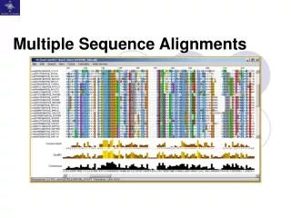
Multiple Sequence Alignments Algorithms
MLAGAN: progressive alignment of DNA Given N sequences, phylogenetic tree Align pairwise, in order of the tree (LAGAN) Human Baboon Mouse Rat
MLAGAN: main steps Given a collection of sequences, and a phylogenetic tree • Find local alignments for every pair of sequences x, y • Find anchors between every pair of sequences, similar to LAGAN anchoring • Progressive alignment • Multi-Anchoring based on reconciling the pairwise anchors • LAGAN-style limited-area DP • Optional refinement steps
MLAGAN: multi-anchoring To anchor the (X/Y), and (Z) alignments: X Z Y Z X/Y Z
Heuristics to improve multiple alignments • Iterative refinement schemes • A*-based search • Consistency • Simulated Annealing • …
Iterative Refinement One problem of progressive alignment: • Initial alignments are “frozen” even when new evidence comes Example: x: GAAGTT y: GAC-TT z: GAACTG w: GTACTG Frozen! Now clear correct y = GA-CTT
Iterative Refinement Algorithm (Barton-Stenberg): • Align most similar xi, xj • Align xk most similar to (xixj) • Repeat 2 until (x1…xN) are aligned • For j = 1 to N, Remove xj, and realign to x1…xj-1xj+1…xN • Repeat 4 until convergence Note: Guaranteed to converge
allow y to vary x,z fixed projection Iterative Refinement For each sequence y • Remove y • Realign y (while rest fixed) z x y
Iterative Refinement Example: align (x,y), (z,w), (xy, zw): x: GAAGTTA y: GAC-TTA z: GAACTGA w: GTACTGA After realigning y: x: GAAGTTA y: G-ACTTA + 3 matches z: GAACTGA w: GTACTGA
Iterative Refinement Example not handled well: x: GAAGTTA y1: GAC-TTA y2: GAC-TTA y3: GAC-TTA z: GAACTGA w: GTACTGA • Realigning any single yi changes nothing
Restricted MDP • Run MDP, restricted to radius R from m z x y Running Time: O(2N RN-1 L)
Tree Refinement Run 3D-DP, restricted to radius R from m, for each tree node z x y Running Time: ~7R2 LN R: Radius L: Alignment Length N: Number of Sequences
A* for Multiple Alignments Review of the A* algorithm h(v) g(v) v GOAL START • g(v) is the cost so far • h(v) is an estimate of the minimum cost from v to GOAL • f(v) ≥ g(v) + h(v) is the minimum cost of a path passing by v • Expand v with the smallest f(v) • Never expand v, if f(v) ≥ shortest path to the goal found so far
A* for Multiple Alignments • Nodes: Cells in the DP matrix • g(v): alignment cost so far • h(v): sum-of-pairs of individual pairwise alignments • Initial minimum alignment cost estimate: sum-of-pairs of global pairwise alignments h(v) g(v) v GOAL START
Consistency – T-Coffee zk z xi x y yj yj’
T – Coffee Layout LALIGN CLUSTALW
Generating Primary Library A A A B B B A A C C B B B C C C ClustalW Primary Library Lalign Primary Library (10 top scoring non–intersecting Local (Global pairwise alignment) (Pairwise alignment) Library has information for each N(N-1)/2 sequence pairs.
Seq A GARFIELD THE LAST FAT CAT Seq B GARFIELD THE FAST CAT - - - Seq A GARFIELD THE LAST FAT CAT Seq D - - - -- - -- THE - - - - FAT CAT Seq B GARFIELD THE FAST CAT Seq D - - - - -- - THE FA-T CAT Prim. Weight = 100 Prim. Weight = 100 Prim. Weight = 88 Seq B GARFIELD THE - - - - FAST CAT Seq C GARFIELD THE VERY FAST CAT Prim. Weight = 100 Seq A GARFIELD THE LAST FA-T CAT Seq C GARFIELD THE VERY FAST --- Prim. Weight = 77 Seq C GARFIELD THE VERY FAST CAT Seq D - - - -- -- - THE - - - - FA-T CAT Prim. Weight = 100 Primary Library
Seq AGARFIELD THE LAST FAT CAT Seq BGARFIELD THE FAST CAT - - - Combining the libraries Primary weight(ClustalW)=88 Primary Weight(Lalign)=88 W(A(G),B(G)) = 88 + 88 = 176 If a pair is duplicated across the two libraries, it is merged into single entry with weight = sum of two weights pairs of residue that did not occur are not present ( weight 0 )
Library Extension • Complete extension requires examination of all triplets. • Not all bring information ( eg. A and B through D ). • Weight of a pair = weights gathered through examination • of all triplets involving that pair.
Running Time • Complexity of entire procedure: O(N2 * L2) + O(N3*L) + O(N3) + O(N*L2) O(N2 L2) - pair-wise library computation O(N3 L) - library extension O(N3) - computation of NJ tree O(N L2) - progressive alignment computation Where: L – average sequence length N – number of sequences
Gene Recognition Credits for slides: Marina Alexandersson Lior Pachter Serge Saxonov
Reading • GENSCAN • EasyGene • SLAM • Twinscan Optional: Chris Burge’s Thesis
DNA transcription RNA translation Protein Gene expression CCTGAGCCAACTATTGATGAA CCUGAGCCAACUAUUGAUGAA PEPTIDE
Gene structure intron1 intron2 exon2 exon3 exon1 transcription splicing translation exon = coding intron = non-coding
Exon 3 Exon 1 Exon 2 Intron 1 Intron 2 5’ 3’ Stop codon TAG/TGA/TAA Start codon ATG Finding genes Splice sites
Approaches to gene finding • Homology • BLAST, Procrustes. • Ab initio • Genscan, Genie, GeneID. • Hybrids • GenomeScan, GenieEST, Twinscan, SGP, ROSETTA, CEM, TBLASTX, SLAM.
intron exon exon intron intergene exon intergene HMMs for gene finding GTCAGAGTAGCAAAGTAGACACTCCAGTAACGC
T A A T A T G T C C A C G G G T A T T G A G C A T T G T A C A C G G G G T A T T G A G C A T G T A A T G A A Exon1 Exon2 Exon3 GHMM for gene finding duration
Better way to do it: negative binomial • EasyGene: Prokaryotic gene-finder Larsen TS, Krogh A • Negative binomial with n = 3
Biology of Splicing (http://genes.mit.edu/chris/)
Consensus splice sites Donor: 7.9 bits Acceptor: 9.4 bits (Stephens & Schneider, 1996) (http://www-lmmb.ncifcrf.gov/~toms/sequencelogo.html)
Donor site 5’ 3’ Position % Splice site detection
Splice Site Models • WMM: weight matrix model = PSSM (Staden 1984) • WAM: weight array model = 1st order Markov (Zhang & Marr 1993) • MDD: maximal dependence decomposition (Burge & Karlin 1997) decision-tree like algorithm to take significant pairwise dependencies into account
atg caggtg ggtgag cagatg ggtgag cagttg ggtgag caggcc ggtgag tga