
Adaptive Image Filtering Using Run-Time Reconfiguration
E N D
Presentation Transcript
Adaptive Image Filtering Using Run-Time Reconfiguration Nitin Srivastava Jerry L. Trahan Ramachandran Vaidyanathan Suresh Rai Department of Electrical and Computer Engineering Louisiana State University
The Problem: Adaptive Image Filtering • A filtering windowmoves over the image pixel by pixel. Window size is usually 33, 55, or 77. • The filter multiplies the intensity values of pixels that the window overlaps with its coefficients and sums the products to produce the new value of the pixel at the center of the window.
Spatially invariant filter — does not change values of its coefficients with the position of the filtering window over the image. • Adaptive filter — adjusts values of its coefficients according to the nature of the image. For instance, handles uniform regions differently than edges.
Use of Run-Time Reconfiguration • For fixed filter coefficients, could use constant coefficient multipliers (KCMs) configured for coefficients. • For adaptive coefficients, we use KCMs configured for pixel values. Flow of data regular, but more involved. • Inspired by 1D adaptive filtering technique of Wojko and ElGindy (RAW’99).
Use of FPGAs • Circuit design tailored to the problem — Filtering exhibits regular, repeated operations, taking an inner product among the same number of elements at each pixel position. • Problem size-specific components and datapaths. • Advantages for this problem even without reconfiguration.
Solution Approach • Gray scale image of size 256256, using a filtering window of size 33. • Can tailor to different image size — changes some register sizes and memory requirements. • Can tailor to different window size — changes memory requirements. • Can extend to video — window is 3D across frames.
Solution Approach, cont. • Basic component is a module. • Sixteen pipelined modules act on 16 contiguous pixels at a time from the same row. • Three sets of three steps each, corresponding to the three rows in a 33 window and the three positions in each row. • For each of these nine steps, a module contributes to one of the nine window computations in which its pixel participates.
Module Algorithm Procedure THREEPIX(r, in, out) Step 0: Adder(r) KCM(r) + in Step 1: Adder(r) KCM(r) + Adder(r1) Step 2: Adder(r) KCM(r) + Adder(r1) out Adder(r) • Contributes to three pixel values on the same row.
Overall Algorithm for i 0 to 255 for k 0 to 255 in steps of 16 for all j, where kjk+15 r = j mod 16 /* module r has v(i, j) */ THREEPIX(r, 0, memory) THREEPIX(r, memory, memory) THREEPIX(r, memory, I/O pins)
filtering window coefficient pixel value To output mux To block memory KCM KCM memory write register zero register module mux KCM output mux 0 previous module next module pipeline register module adder memory read register From block memory step counter Module
First vantage point: one module
7,25 7,23 7,24 7,26 7,27 5,22 5,26 5,27 5,28 5,29 5,23 5,24 5,25 6,22 6,23 6,24 6,25 6,26 6,27 6,28 6,29 7,22 7,28 7,29 8,22 8,23 8,24 8,25 8,26 8,27 8,28 8,29 9,22 9,23 9,24 9,25 9,26 9,27 9,28 9,29
block memories block memory block memory block memory 5,22 5,26 5,27 5,28 5,29 5,23 5,24 5,25 6,23 6,27 6,22 6,24 6,25 6,26 6,28 6,29 7,22 7,26 7,23 7,24 7,25 7,27 7,28 7,29 8,24 8,22 8,23 8,25 8,26 8,27 8,28 8,29 9,22 9,23 9,24 9,25 9,26 9,27 9,28 9,29
v[7,23] v[7,24] v[7,25] v[7,26] v[7,27] 0 0 0 0 0 pd[8,27,-1,-1] pd[8,24,-1,-1] pd[8,25,-1,-1] pd[8,26,-1,-1] pd[8,28,-1,-1] pd[8,26,-1,0]
block memories block memory block memory block memory 5,22 5,22 5,26 5,26 5,27 5,27 5,28 5,28 5,29 5,29 5,23 5,23 5,24 5,24 5,25 5,25 6,23 6,23 6,27 6,27 6,22 6,22 6,24 6,24 6,25 6,25 6,26 6,26 6,28 6,28 6,29 6,29 7,22 7,22 7,26 7,26 7,23 7,23 7,24 7,24 7,25 7,25 7,27 7,27 7,28 7,28 7,29 7,29 8,24 8,24 8,22 8,22 8,23 8,23 8,25 8,25 8,26 8,26 8,27 8,27 8,28 8,28 8,29 8,29 9,22 9,22 9,23 9,23 9,24 9,24 9,25 9,25 9,26 9,26 9,27 9,27 9,28 9,28 9,29 9,29 Nitin: Slide added
v[7,23] v[7,24] v[7,25] v[7,26] v[7,27] 0 0 0 0 0 pd[8,27,-1,-1] pd[8,24,-1,-1] pd[8,25,-1,-1] pd[8,26,-1,-1] pd[8,28,-1,-1] pd[8,25,-1,0] pd[8,24,-1,0] pd[8,26,-1,0] pd[8,27,-1,0] pd[8,23,-1,0] pd[8,25,-1,1]
rs(-1)[8,24] block memories block memory 9 block memory block memory 5,22 5,26 5,27 5,28 5,29 5,23 5,24 5,25 6,23 6,27 6,22 6,24 6,25 6,26 6,28 6,29 7,22 7,26 7,23 7,24 7,25 7,27 7,28 7,29 8,24 8,22 8,23 8,25 8,26 8,27 8,28 8,29 9,22 9,23 9,24 9,25 9,26 9,27 9,28 9,29
v[7,23] v[7,24] v[7,25] v[7,26] v[7,27] 0 0 0 0 0 pd[8,27,-1,-1] pd[8,24,-1,-1] pd[8,25,-1,-1] pd[8,26,-1,-1] pd[8,28,-1,-1] pd[8,25,-1,0] pd[8,24,-1,0] pd[8,26,-1,0] pd[8,27,-1,0] pd[8,23,-1,0] pd[8,22,-1,1] pd[8,24,-1,1] pd[8,25,-1,1] pd[8,26,-1,1] pd[8,23,-1,1] rs(-1)[8,24]
newv[6,24] block memories block memory 9 block memory block memory 11 rs(-1)[8,24] rs(-1)[7,26] rs(-1)[7.24]+ rs(0)[7,24] rs(-1)[6,26]+ rs(0)[6.26] 5,22 5,26 5,27 5,28 5,29 5,23 5,24 5,25 6,27 6,23 6,22 6,24 6,25 6,26 6,28 6,29 7,22 7,26 7,23 7,24 7,25 7,27 7,28 7,29 8,24 8,22 8,23 8,25 8,26 8,27 8,28 8,29 9,22 9,23 9,24 9,25 9,26 9,27 9,28 9,29
v[7,23] v[7,24] v[7,25] v[7,26] v[7,27] 0 0 0 0 0 pd[8,27,-1,-1] pd[8,24,-1,-1] pd[8,25,-1,-1] pd[8,26,-1,-1] pd[8,28,-1,-1] pd[8,25,-1,0] pd[8,24,-1,0] pd[8,26,-1,0] pd[8,27,-1,0] pd[8,23,-1,0] pd[8,22,-1,1] rs(-1)[7,26] pd[8,24,-1,1] pd[8,25,-1,1] pd[8,26,-1,1] pd[8,23,-1,1] rs(-1)[8,24] pd[7,26,0,-1] pd[7,28,0,-1] pd[7,25,0,-1] pd[7,27,0,-1] pd[7,24,0,-1] pd[7,24,0,0] pd[7,25,0,0] pd[7,26,0,0] pd[7,27,0,0] pd[7,23,0,0] pd[7,23,0,1] pd[7,25,0,1] pd[7,26,0,1] pd[7,24,0,1] rs(-1)[6,26]+ rs(0)[6,26] pd[7,22,0,1] rs(-1)[7,24]+rs(0)[7,24] pd[6,26,1,-1] pd[6,27,1,-1] pd[6,28,1,-1] pd[6,25,1,-1] pd[6,24,1,-1] pd[6,25,1,0] pd[6,24,1,0] pd[6,26,1,0] pd[6,27,1,0] pd[6,23,1,0] pd[6,24,1,1] pd[6,25,1,1] pd[6,26,1,1] pd[6,23,1,1] pd[6,22,1,1] newv[6,24]
Second vantage point: one pixel
5,22 5,26 5,27 5,28 5,29 5,23 5,24 5,25 6,23 6,24 6,25 6,26 6,27 6,22 6,28 6,29 7,22 7,23 7,24 7,25 7,26 7,27 7,28 7,29 8,22 8,23 8,24 8,25 8,26 8,27 8,28 8,29 9,22 9,23 9,24 9,25 9,26 9,27 9,28 9,29
v[6,23] v[6,24] v[6,25] v[6,26] v[6.27] 0 0 0 0 0 pd[7,24,-1,-1] pd[7,25,-1,-1] pd[7,26,-1,-1] pd[7,27,-1,-1] pd[7,28 –1,-1]
v[6,23] v[6,24] v[6,25] v[6,26] v[6.27] 0 0 0 0 0 pd[7,24,-1,-1] pd[7,25,-1,-1] pd[7,26,-1,-1] pd[7,27,-1,-1] pd[7,28,-1,-1] pd[7,24,-1,0] pd[7,25,-1,0] pd[7,26,-1,0] pd[7,27,-1,0] pd[7,23,-1,0]
v[6,23] v[6,24] v[6,25] v[6,26] v[6.27] 0 0 0 0 0 pd[7,27,-1,-1] pd[7,24,-1,-1] pd[7,25,-1,-1] pd[7,26,-1,-1] pd[7,28,-1,-1] pd[7,24,-1,0] pd[7,25,-1,0] pd[7,26,-1,0] pd[7,27,-1,0] pd[7,23,-1,0] pd[7,24,-1,1] pd[7,23,-1,1] pd[7,25,-1,1] pd[7,26,-1,1] pd[7,22,-1,1] rs(-1)[7,25]
v[8,23] v[8,24] v[8,25] v[8,26] v[8,27] 0 0 0 0 0 pd[9,27,-1,-1] pd[9,24,-1,-1] pd[9,25,-1,-1] pd[9,26,-1,-1] pd[9,28,-1,-1] pd[9,24,-1,0] pd[9,25,-1,0] pd[9,26,-1,0] pd[9,27,-1,0] pd[9,23,-1,0] pd[9,24,-1,1] pd[9,23,-1,1] pd[9,25,-1,1] pd[9,26,-1,1] pd[9,22,-1,1] pd[8,26,0,-1] pd[8,27,0,-1] pd[8,28,0,-1] pd[8,25,0,-1] pd[8,24,0,-1] pd[8,24,0,0] pd[8,25,0,0] pd[8,26,0,0] pd[8,27,0,0] pd[8,23,0,0] pd[8,25,0,1] pd[8,26,0,1] pd[8,24,0,1] pd[8,23,0,1] pd[8,22,0,1] rs(-1)[7,25]+ rs(0)[7,25] pd[7,26,1,-1] pd[7,28,1,-1] pd[7,27,1,-1] pd[7,25,1,-1] pd[7,24,1,-1] pd[7,25,1,0] pd[7,24,1,0] pd[7,27,1,0] pd[7,26,1,0] pd[7,23,1,0] pd[7,26,1,1] pd[7,25,1,1] pd[7,22,1,1] pd[7,23,1,1] pd[7,24,1,1] newv[7,25]
Evaluation • Xilinx Virtex-E FPGA XCV200E • Number of CLB slices required = 492 • Clock frequency = 101.9 MHz • Time spent in filtering a 256256 image = 642 s
System description Running time Speedup 866 MHz Pentium III system 20 ms 31 400 MHz Sun Ultra 5 system 53 ms 84 Comparison