An Overview of Network Routing Protocols: Concepts, Challenges, and Techniques
760 likes | 906 Vues
This document provides a comprehensive overview of routing in network communications, distinguishing between routing, forwarding, and bridging. It explores key concepts like distance-vector and link-state routing, addressing scalability, and examines prominent protocols such as OSPF and BGP. The discussion includes inter-domain routing issues, data-plane versus control-plane functions, and challenges related to consistency, completeness, and scalability in large networks. The routing model illustrated emphasizes dynamic routing within and between autonomous systems, showcasing the fundamental techniques and considerations for effective network routing.

An Overview of Network Routing Protocols: Concepts, Challenges, and Techniques
E N D
Presentation Transcript
Routing: Overview and Key Protocols Shivkumar Kalyanaraman Rensselaer Polytechnic Institute shivkuma@ecse.rpi.edu Based in part upon slides of Prof. Raj Jain (OSU), S. Keshav (Cornell), J. Kurose (U Mass), Noel Chiappa (MIT), Tim Griffin (AT&T), Ion Stoica (UCB),
Overview • Routing vs Forwarding vs Bridging • Distance vector vs Link state routing • Addressing and Routing: Scalability • OSPF, RIP protocols • Inter-domain Routing Issues • BGP protocol
Routing vs. Forwarding • Forwarding: select an output port based on destination address and routing table • Data-plane function • Often implemented in hardware • Routing: process by which routing table is built.. • … so that the series of local forwarding decisions takes the packet to the destination with high probability, and …(reachability condition) • … the path chosen/resources consumed by the packet is efficient in some sense… (optimality and filtering condition) • Control-plane function • Implemented in software
Forwarding Table • Can display forwarding table using “netstat -rn” • Sometimes called “routing table” DestinationGatewayFlags RefUseInterface 127.0.0.1 127.0.0.1 UH 0 26492 lo0 192.168.2. 192.168.2.5 U 2 13 fa0 193.55.114. 193.55.114.6 U 3 58503 le0 192.168.3. 192.168.3.5 U 2 25 qaa0 224.0.0.0 193.55.114.6 U 3 0 le0 default 193.55.114.129 UG 0 143454
H H Gateway Router Bridge/Switch Repeater/Hub Interconnection Devices Extended LAN =Broadcast domain LAN= CollisionDomain B H H Router Application Application Transport Transport Network Network Datalink Datalink Physical Physical
Routing problem • Collect, process, and condense global state into local forwarding information • Global state • inherently large • dynamic • hard to collect • Hard issues: • consistency, completeness, scalability • Impact of resource needs of sessions
Consistency • Defn: A series of independent local forwarding decisions must lead to connectivity between any desired (source, destination) pair in the network. • If the states are inconsistent, the network is said not to have “converged” to steady state (I.e. is in a transient state) • Inconsistency leads to loops, wandering packets etc • In general a part of the routing information may be consistent while the rest may be inconsistent. • Large networks => inconsistency is a scalability issue. • Consistency can be achieved in two ways: • Fully distributed approach: a consistency criterion or invariant across the states of adjacent nodes • Signaled approach: the signaling protocol sets up local forwarding information along the path.
Completeness • Defn: The network as a whole and every node has sufficient information to be able to compute all paths. • In general, with more information available locally, routing algorithms tend to converge faster, because the chances of inconsistency reduce. • But this means that more distributed state must be collected at each node and processed. • The demand for completeness also limits the scalability of the algorithm. • Since both consistency and completeness pose scalability problems, large networks have to be structured hierarchically and abstract entire networks as a single node.
Internet Routing Model • 2 key features: • Dynamic routing • Intra- and Inter-AS routing, AS = locus of admin control • Internet organized as “autonomous systems” (AS). • AS is internally connected • Interior Gateway Protocols (IGPs) within AS. • Eg: RIP, OSPF, HELLO • Exterior Gateway Protocols (EGPs) for AS to AS routing. • Eg: EGP, BGP-4
c b b c a network layer inter-AS, intra-AS routing in gateway A.c link layer physical layer A.c A.a C.b B.a Intra-AS and Inter-AS routing • Gateways: • perform inter-AS routing amongst themselves • perform intra-AS routers with other routers in their AS b a a C B d A
Inter-AS routing between A and B b c a a C b B b a c d Host h1 A A.a A.c C.b B.a Intra-AS and Inter-AS routing: Example Host h2 Intra-AS routing within AS B Intra-AS routing within AS A
Basic Dynamic Routing Methods • Source-based: source gets a map of the network, • source finds route, and either • signals the route-setup (eg: ATM approach) • encodes the route into packets (inefficient) • Link state routing: per-link information • Get map of network (in terms of link states) at all nodes and find next-hops locally. • Maps consistent => next-hops consistent • Distance vector:per-node information • At every node, set up distance signposts to destination nodes (a vector) • Setup this by peeking at neighbors’ signposts.
DV & LS: consistency criterion • The subset of a shortest path is also the shortest path between the two intermediate nodes. • Corollary: • If the shortest path from node i to node j, with distance D(i,j) passes through neighbor k, with link cost c(i,k), then: D(i,j) = c(i,k) + D(k,j) j D(k,j) i c(i,k) k
Distance Vector DV = Set (vector) of Signposts, one for each destination
1 1 7 A A A D D E B B E B E C C 7 7 2 8 8 1 1 1 2 2 Example network A’s 1-hop view (After 1st iteration) A’s 2-hop view (After 2nd Iteration) Distance Vector (DV) Approach Consistency Condition: D(i,j) = c(i,k) + D(k,j) • The DV (Bellman-Ford) algorithm evaluates this recursion iteratively. • In the mth iteration, the consistency criterion holds, assuming that each node sees all nodes and links m-hops (or smaller) away from it (i.e. an m-hop view)
1 1 7 A A A D D E B B E B E C C 7 7 2 8 8 1 1 1 2 2 Example network A’s 1-hop view (After 1st iteration) A’s 2-hop view (After 2nd Iteration) Distance Vector (DV) Example • A’s distance vector D(A,*): • After Iteration 1 is: [0, 7, INFINITY, INFINITY, 1] • After Iteration 2 is: [0, 7, 8, 3, 1] • After Iteration 3 is: [0, 7, 5, 3, 1] • After Iteration 4 is: [0, 6, 5, 3, 1]
Link State (LS) Approach • The link state (Dijkstra) approach is iterative, but it pivots around destinations j, and their predecessors k = p(j) • Observe that an alternative version of the consistency condition holds for this case: D(i,j) = D(i,k) + c(k,j) • Each node i collects all link states c(*,*) first and runs the complete Dijkstra algorithm locally. j c(k,j) i D(i,k) k
5 3 5 2 2 1 3 1 2 1 A D E B F C Dijkstra’s algorithm: example D(B),p(B) 2,A 2,A 2,A D(D),p(D) 1,A D(C),p(C) 5,A 4,D 3,E 3,E D(E),p(E) infinity 2,D Step 0 1 2 3 4 5 set N A AD ADE ADEB ADEBC ADEBCF D(F),p(F) infinity infinity 4,E 4,E 4,E The shortest-paths spanning tree rooted at A is called an SPF-tree
Topology information is flooded within the routing domain Best end-to-end paths are computed locally at each router. Best end-to-end paths determine next-hops. Based on minimizing some notion of distance Works only if policy is shared and uniform Examples: OSPF, IS-IS Each router knows little about network topology Only best next-hops are chosen by each router for each destination network. Best end-to-end paths result from composition of all next-hop choices Does not require any notion of distance Does not require uniform policies at all routers Examples: RIP, BGP Summary: Distributed Routing Techniques Link State Vectoring
RIP: Routing Information Protocol • Uses hop count as metric (max: 16 is infinity) • Tables (vectors) “advertised” to neighbors every 30 s. • Each advertisement: upto 25 entries • No advertisement for 180 sec: neighbor/link declared dead • routes via neighbor invalidated • new advertisements sent to neighbors (Triggered updates) • neighbors in turn send out new advertisements (if tables changed) • link failure info quickly propagates to entire net • poison reverse used to prevent ping-pong loops (infinite distance = 16 hops)
RIPv1 Problems (Continued) • Split horizon/poison reverse does not guarantee to solve count-to-infinity problem • 16 = infinity => RIP for small networks only! • Slow convergence • Broadcasts consume non-router resources • RIPv1 does not support subnet masks (VLSMs) • No authentication
RIPv2 • Why ? Installed base of RIP routers • Provides: • VLSM support • Authentication • Multicasting • “Wire-sharing” by multiple routing domains, • Tags to support EGP/BGP routes. • Uses reserved fields in RIPv1 header. • First route entry replaced by authentication info.
Link State Protocols • Key: Create a network “map” at each node. • 1. Node collects the state of its connected links and forms a “Link State Packet” (LSP) • 2. Flood LSP => reaches every other node in the network and everyone now has a network map. • 3. Given map, run Dijkstra’s shortest path algorithm (SPF) => get paths to all destinations • 4. Routing table = next-hops of these paths. • 5. Hierarchical routing: organization of areas, and filtered control plane information flooded.
Topology Dissemination • A.k.a LSP distribution • 1. Flood LSPs on links except incoming link • Require at most 2E transfers for n/w with E edges • 2. Sequence numbers to detect duplicates • Why? Routers/links may go down/up • Issue: wrap-around, larger sequence number is not the most recent!
Topology Dissemination (Continued) • Checksum field: • Drop packet if in error, get retransmission from neighbor • Age field (similar to TTL) • Number of seconds since LSA originated • Periodically incremented after acceptance • Originating router refreshes LSA after 30 min • Delete if Age = MaxAge • Low age field + large seq # => that LSA is flapping or frequently changing …
Recovering from a partition • On partition, LSP databases can get out of synch • Databases described by database descriptor records • Routers on each side of a newly restored link talk to each other to update databases (determine missing and out-of-date LSPs) => selective synchronization
Inter-Domain Routing: Big Picture Large ISP Large ISP Stub Small ISP Dial-Up ISP Access Network Stub Stub Large number of diverse networks
Requirements for Inter-AS Routing • Should scale for the size of the global Internet. • Focus on reachability, not optimality • Use address aggregation techniques to minimize core routing table sizes and associated control traffic • At the same time, it should allow flexibility in topological structure (eg: don’t restrict to trees etc) • Allow policy-based routing between autonomous systems • Policy refers to arbitrary preference among a menu of available routes (based upon routes’ attributes) • Fully distributed routing (as opposed to a signaled approach) is the only possibility. • Extensible to meet the demands for newer policies.
R R2 R1 R3 Who speaks Inter-AS routing? AS2 AS1 BGP border router internal router • Two types of routers • Border router(Edge), Internal router(Core) • Two border routers of different ASes will have a BGP session
provider customer IP traffic Customers and Providers provider customer Customer pays provider for access to the Internet
Nontransit vs. Transit ASes Internet Service providers (ISPs) have transit networks ISP 2 ISP 1 NET A Nontransit AS might be a corporate or campus network. Could be a “content provider” Traffic NEVER flows from ISP 1 through NET A to ISP 2
peer peer provider customer The Peering Relationship Peers provide transit between their respective customers Peers do not provide transit between peers Peers (often) do not exchange $$$ traffic allowed traffic NOT allowed
BGP-4 • BGP = Border Gateway Protocol • Is a Policy-Based routing protocol • Is the de facto EGP of today’s global Internet • Relatively simple protocol, but configuration is complex and the entire world can see, and be impacted by, your mistakes. • 1989 : BGP-1 [RFC 1105] • Replacement for EGP (1984, RFC 904) • 1990 : BGP-2 [RFC 1163] • 1991 : BGP-3 [RFC 1267] • 1995 : BGP-4 [RFC 1771] • Support for Classless Interdomain Routing (CIDR)
BGP Operations (Simplified) Establish session on TCP port 179 AS1 BGP session Exchange all active routes AS2 While connection is ALIVE exchange route UPDATE messages Exchange incremental updates
Four Types of BGP Messages • Open : Establish a peering session. • Keep Alive : Handshake at regular intervals. • Notification : Shuts down a peering session. • Update : Announcing new routes or withdrawing previously announced routes. announcement = prefix + attributes values
Two Types of BGP Neighbor Relationships • External Neighbor (eBGP) in a different Autonomous Systems • Internal Neighbor (iBGP) in the same Autonomous System AS1 iBGP is routed (using IGP!) eBGP iBGP AS2
IGP: Interior Gateway Protocol. Examples: IS-IS, OSPF I-BGP R R1 R4 R5 R2 R3 AS1 announce B AS3 border router internal router B I-BGP and E-BGP IGP A E-BGP AS2
IBGP vs EBGP • I-BGP nodes: typically ABRs, or other nodes where default routes terminate • I-BGP peering sessions between every pair of routers within an AS: full mesh. Physical link A IBGP session D C B AS1
Route Reflection 128.23.0.0/16 RR2 RR-C4 RR-C1 RR1 RR3 RR-C3 RR-C2 AS1 ER EBGP 10.0.0.0/24 AS2 IBGP
AS Confederations • Divide and conquer: Divides a large AS into sub-ASs Sub-AS 11 10 14 13 12 R1 AS-1 R2
Address Aggregation: CIDR 204.71.0.0 204.71.0.0 204.71.1.0 Global Internet Routing Mesh Service Provider 204.71.1.0 204.71.2.0 204.71.2.0 …...……. …...……. 204.71.255.0 204.71.255.0 Inter-domain Routing Without CIDR 204.71.0.0 204.71.1.0 Global Internet Routing Mesh Service Provider 204.71.2.0 204.71.0.0/16 …...……. 204.71.255.0 Inter-domain Routing With CIDR
00001100 00000100 00000000 00000000 11111111 11111110 00000000 00000000 RFC 1519: Classless Inter-Domain Routing (CIDR) Pre-CIDR: Network ID ended on 8-, 16, 24- bit boundary CIDR:Network ID can end at any bit boundary IP Address : 12.4.0.0 IP Mask: 255.254.0.0 Address Mask Network Prefix for hosts Usually written as 12.4.0.0/15, a.k.a “supernetting”
Prefix Next Hop Interface 0.0.0.0/0 10.14.11.33 ATM 5/0/9 12.0.0.0/8 10.14.22.19 ATM 5/0/8 12.4.0.0/15 10.1.3.77 Ethernet 0/1/3 12.5.8.0/23 attached Serial 1/0/7 IP Forwarding Table Longest Prefix Match (Classless) Forwarding Destination =12.5.9.16 ------------------------------- payload OK better even better best!
What is Routing Policy • Policy refers to arbitrary preference among a menu of available routes (based upon routes’ attributes) • Public description of the relationship between external BGP peers • Can also describe internal BGP peer relationship • Eg: Who are my BGP peers • What routes are • Originated by a peer • Imported from each peer • Exported to each peer • Preferred when multiple routes exist • What to do if no route exists?
BGP Route Processing Apply Policy = filter routes & tweak attributes Apply Policy = filter routes & tweak attributes Receive BGP Updates Based on Attribute Values Best Routes Transmit BGP Updates Apply Import Policies Best Route Selection Best Route Table Apply Export Policies Install forwarding Entries for best Routes. IP Forwarding Table
Adj RIB In Main BGP RIB Adj RIB Out Incom- ing Outgo- ing IGPs Main RIB/ FIB Static & HW Info Policy Implementation Flow