Calibration and Static Response
This text explores the principles of calibration and the response characteristics of measurement systems. It highlights how systems respond to inputs, emphasizing differences in output frequency, amplitude, and phase lag. Calibration is defined as the comparison of measured values to true values, with discussions on absolute and relative error. Static and dynamic responses are examined, along with examples of first-order and zero-order systems. Key concepts like static sensitivity and conservation of energy in thermal systems are also covered, providing a comprehensive overview of measurement system behavior.

Calibration and Static Response
E N D
Presentation Transcript
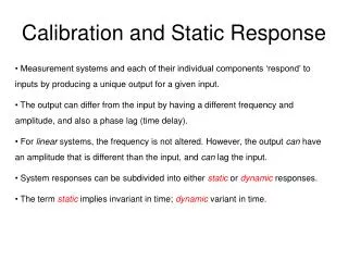
Calibration and Static Response • Measurement systems and each of their individual components ‘respond’ to inputs by producing a unique output for a given input. • The output can differ from the input by having a different frequency and amplitude, and also a phase lag (time delay). • For linear systems, the frequency is not altered. However, the output can have an amplitude that is different than the input, and can lag the input. • System responses can be subdivided into either static or dynamic responses. • The term static implies invariant in time; dynamic variant in time.
Figure 5.1 A Static Calibration • The slope of the static calibration curve is the staticsensitivity, K. • K=K(x) → many different values of K for a given curve. • Usually a high static sensitivity is desired (this leads to a lower x-from-y uncertainty).
Calibration Terms • Calibration is the comparison of a measured value to a known, • much more accurate value, which is called the true value. • The absolute error is the difference between the measured and true values. • The relative error is the ratio of the absolute error over the true value. • The accuracy of the calibration equals 1 - relative error. • When a calibration consists of a number of comparisons, the maximum • relative error often is used to characterize the calibration.
Dynamic Response Characterization • The output, y(t), of a linear system can be determined by • by solving the linear ordinary differential equation (ODE) • in which the a’s are constant coefficients, n the order of the • system, and F(t) the forcing function. • y(t) can represent a physical variable that varies in time, • such as pressure, temperature, velocity, … • The exact ODE that describes the system is derived from • a conservation law.
This is known as Fourier’s law. Example First-Order System • Consider the response of a bulb thermometer • that is immersed from room air into hot water. • Heat is transferred from the hotter water through • glass wall into the cooler liquid inside the bulb. • This thermal energy transfer is governed by the first law of thermodynamics. E = total energy (J); Q = heat transfer (J); t = time (s) • Heat is transferred convectively to the glass from the hot water as h = heat transfer coefficient (W / [m2K]); A = surface area of heat transfer
Assume that all of the heat transferred from the hot water through the glass • reaches the liquid inside the bulb, thereby increasing the temperature of the • liquid. Conservation of energy requires that m = mass of the liquid (kg); Cv = specific heat at constant volume of the liquid (J / [kg K]) • Combining the previous equations gives • This is a linear, first-order ordinary differential equation, which is of the form Here, y = T, K = 1, Thw = F(t), and t = mCv/hA.
For a zero-order system (n=0), Examples: strain gage, pitot-static tube • For a first-order system (n=1), Examples: thermometer, RC circuit • For a second-order system (n=2), Examples: pressure transducer, accelerometer, RLC circuit Lower-Order Systems