Continuous heterogeneity
Continuous heterogeneity. Danielle Dick & Sarah Medland Boulder Twin Workshop March 2006. Ways to Model Heterogeneity in Twin Data. Multiple Group Models Sex Effects Young/Old cohorts. Problem:. Many variables of interest do not fall into groups Age Socioeconomic status

Continuous heterogeneity
E N D
Presentation Transcript
Continuous heterogeneity Danielle Dick & Sarah Medland Boulder Twin Workshop March 2006
Ways to Model Heterogeneity in Twin Data • Multiple Group Models • Sex Effects • Young/Old cohorts
Problem: • Many variables of interest do not fall into groups • Age • Socioeconomic status • Regional alcohol sales • Parental warmth • Parental monitoring • Grouping these variables into high/low categories loses a lot of information
‘Definition variables’ in Mx • General definition: Definition variables are variables that may vary per subject and that are not dependent variables • In Mx:The specific value of the def var for a specific individual is read into a matrix in Mx when analyzing the data of that particular individual
‘Definition variables’ in Mx create dynamic var/cov structure • Common uses: 1. As covariates/effects on the means (e.g. age and sex) 2. To model changes in variance components as function of some variable (e.g., age, SES, etc)
Cautionary note about definition variables • Def var should not be missing if dependent is not missing • Def var should not have the same missing value as dependent variable (e.g., use -2.00 for def var, -1.00 for dep var)
Definition variables used as covariates General model with age and sex as covariates: yi = + 1(agei) + 2 (sexi) + Where yi is the observed score of individual i, is theintercept or grand mean, 1is the regression weight of age, ageiis the age of individual i, 2 is the deviation of males (if sex is coded 0= female; 1=male), sexiis the sex ofindividual i, and is the residual that is not explained by the covariates (and can be decomposed further into ACE etc).
Standard model • Means vector • Covariance matrix
Allowing for a main effect of X • Means vector • Covariance matrix
! Basic model + main effect of a definition variable G1: Define Matrices Data Calc NGroups=3 Begin Matrices; X full 1 1 free !genetic influences Y full 1 1 free !common environmental influences Z full 1 1 free !unique environmental influences M full 1 1 free ! grand mean B full 1 1 free ! moderator-linked means model H full 1 1 !coefficient for DZ genetic relatedness R full 1 1 ! twin 1 moderator (definition variable) S full 1 1 ! twin 2 moderator (definition variable) End Matrices; Ma M 0 Ma B 0 Ma X 1 Ma Y 1 Ma Z 1 Matrix H .5 Options NO_Output End
Select phenoTw1, phenoTw2, modTw1, modTw2 G2: MZ Data NInput_vars=6 NObservations=0 Missing =-999 RE File=f1.dat Labels id zyg p1 p2 m1 m2 Select if zyg = 1 / Select p1 p2 m1 m2 / Definition m1 m2 / Matrices = Group 1 Means M + B*R | M + B*S / Covariance X*X' + Y*Y' + Z*Z' | X*X' + Y*Y' _ X*X' + Y*Y' | X*X' + Y*Y' + Z*Z' / !twin 1 moderator variable Specify R -1 !twin 2 moderator variable Specify S -2 End
G2: MZ Data NInput_vars=6 NObservations=0 Missing =-999 RE File=f1.dat Labels id zyg p1 p2 m1 m2 Select if zyg = 1 / Select p1 p2 m1 m2 / Definition m1 m2 / Matrices = Group 1 Means M + B*R | M + B*S / Covariance X*X' + Y*Y' + Z*Z' | X*X' + Y*Y' _ X*X' + Y*Y' | X*X' + Y*Y' + Z*Z' / !twin 1 moderator variable Specify R -1 !twin 2 moderator variable Specify S -2 End Tell MX modTw1, modTw2 are Definition Variables
G2: MZ Data NInput_vars=6 NObservations=0 Missing =-999 RE File=f1.dat Labels id zyg p1 p2 m1 m2 Select if zyg = 1 / Select p1 p2 m1 m2 / Definition m1 m2 / Matrices = Group 1 Means M + B*R | M + B*S / Covariance X*X' + Y*Y' + Z*Z' | X*X' + Y*Y' _ X*X' + Y*Y' | X*X' + Y*Y' + Z*Z' / !twin 1 moderator variable Specify R -1 !twin 2 moderator variable Specify S -2 End
G3: DZ Data NInput_vars=6 NObservations=0 Missing =-999 RE File=f1.dat Labels id zyg p1 p2 m1 m2 Select if zyg = 2 / Select p1 p2 m1 m2 / Definition m1 m2 / Matrices = Group 1 Means M + B*R | M + B*S / Covariance X*X' + Y*Y' + Z*Z' | H@X*X' + Y*Y' _ H@X*X' + Y*Y' | X*X' + Y*Y' + Z*Z' / !twin 1 moderator variable Specify R -1 !twin 2 moderator variable Specify S -2 End
MATRIX X This is a FULL matrix of order 1 by 1 1 1 1.3228 MATRIX B This is a FULL matrix of order 1 by 1 1 1 0.3381 MATRIX Y This is a FULL matrix of order 1 by 1 1 1 1.1051 MATRIX Z This is a FULL matrix of order 1 by 1 1 1 0.9728 MATRIX M This is a FULL matrix of order 1 by 1 1 1 0.1035 Your model has 5 estimated parameters and 800 Observed statistics -2 times log-likelihood of data >>> 3123.925 Degrees of freedom >>>>>>>>>>>>>>>> 795
MATRIX X This is a FULL matrix of order 1 by 1 1 1 1.3078 MATRIX B This is a FULL matrix of order 1 by 1 1 1 0.0000 MATRIX Y This is a FULL matrix of order 1 by 1 1 1 1.1733 MATRIX Z This is a FULL matrix of order 1 by 1 1 1 0.9749 MATRIX M This is a FULL matrix of order 1 by 1 1 1 0.1069 Your model has 4 estimated parameters and 800 Observed statistics -2 times log-likelihood of data >>> 3138.157 Degrees of freedom >>>>>>>>>>>>>>>> 796
Model-fitting approach to GxE A C E A C E c a e a c e m m Twin 1 Twin 2 M M
Adding Covariates to Means Model A C E A C E c a e a c e m+MM1 m+MM2 Twin 1 Twin 2 M M
‘Definition variables’ in Mx create dynamic var/cov structure • Common uses: 1. As covariates/effects on the means (e.g. age and sex) 2. To model changes in variance components as function of some variable (e.g., age, SES, etc)
Model-fitting approach to GxE A C E A C E c a+XM e a+XM c e m+MM1 m+MM2 Twin 1 Twin 1 Twin 2 Twin 2 M M
Individual specific moderators A C E A C E c a+XM1 e a+XM2 c e m+MM1 m+MM2 Twin 1 Twin 1 Twin 2 Twin 2 M M
E x E interactions A C E A C E c+YM1 c+YM2 a+XM1 a+XM2 e+ZM1 e+ZM2 m+MM1 m+MM2 Twin 1 Twin 1 Twin 2 Twin 2 M M
ACE - XYZ - M A C E A C E c+YM1 c+YM2 a+XM1 a+XM2 e+ZM1 e+ZM2 m+MM1 m+MM2 Twin 1 Twin 2 M M Main effects and moderating effects
Definition Variables in Mx GUI X a M1 Dick et al., 2001
Classic Twin Model: Var (P) = a2 + c2 + e2 • Moderation Model: Var (P) = (a + βXM)2 + (c + βYM)2 + (e + βZM)2 Purcell 2002, Twin Research
Var (T) = (a + βXM)2 + (c + βYM)2 (e + βZM)2 Where M is the value of the moderator and Significance of βX indicates genetic moderation Significance of βY indicates common environmental moderation Significance of βZ indicates unique environmental moderation BM indicates a main effect of the moderator on the mean
Plotting VCs as Function of Moderator • For the additive genetic VC, for example • Given a, (estimated in Mx model) and a range of values for the moderator variable • For example, a = 0.5, = -0.2 and M ranges from -2 to +2
Model-fitting approach to GxE C Component of variance A E Moderator variable
Matrix Letters as Specified in Mx Script A C E A C E c+YM1 c+YM2 a+XM1 a+XM2 Y+U*R Y+U*S e+ZM1 e+ZM2 X+T*R X+T*S Z+V*S Z+V*R Twin 1 Twin 2 M M m+MM2 m+MM1 M+B*S M+B*R
! GxE - Basic model G1: Define Matrices Data Calc NGroups=3 Begin Matrices; X full 1 1 free Y full 1 1 free Z full 1 1 free T full 1 1 free ! moderator-linked A component U full 1 1 free ! moderator-linked C component V full 1 1 free ! moderator-linked E component M full 1 1 free ! grand mean B full 1 1 free ! moderator-linked means model H full 1 1 R full 1 1 ! twin 1 moderator (definition variable) S full 1 1 ! twin 2 moderator (definition variable) End Matrices; Ma T 0 Ma U 0 Ma V 0 Ma M 0 Ma B 0 Ma X 1 Ma Y 1 Ma Z 1 Matrix H .5 Options NO_Output End
G2: MZ Data NInput_vars=6 NObservations=0 Missing =-999 RE File=f1.dat Labels id zyg p1 p2 m1 m2 Select if zyg = 1 / Select p1 p2 m1 m2 / Definition m1 m2 / Matrices = Group 1 Means M + B*R | M + B*S / Covariance (X+T*R)*(X+T*R) + (Y+U*R)*(Y+U*R) + (Z+V*R)*(Z+V*R) | (X+T*R)*(X+T*S) + (Y+U*R)*(Y+U*S) _ (X+T*S)*(X+T*R) + (Y+U*S)*(Y+U*S) | (X+T*S)*(X+T*S) + (Y+U*S)*(Y+U*S) + (Z+V*S)*(Z+V*S) / !twin 1 moderator variable Specify R -1 !twin 2 moderator variable Specify S -2 Options NO_Output End
G2: DZ Data NInput_vars=6 NObservations=0 Missing =-999 RE File=f1.dat Labels id zyg p1 p2 m1 m2 Select if zyg = 1 / Select p1 p2 m1 m2 / Definition m1 m2 / Matrices = Group 1 Means M + B*R | M + B*S / Covariance (X+T*R)*(X+T*R) + (Y+U*R)*(Y+U*R) + (Z+V*R)*(Z+V*R) | H@(X+T*R)*(X+T*S) + (Y+U*R)*(Y+U*S) _ H@(X+T*S)*(X+T*R) + (Y+U*S)*(Y+U*S) | (X+T*S)*(X+T*S) + (Y+U*S)*(Y+U*S) + (Z+V*S)*(Z+V*S) / !twin 1 moderator variable Specify R -1 !twin 2 moderator variable Specify S -2 Options NO_Output End
Practical • Cohort (young/old) model using definition variables (coded 0/1) • Extension to continuous age
Cohort Moderation Younger Cohort Older Cohort
Cohort Moderation Same fit as 4 group script Younger Cohort Older Cohort
Your task • Add tests to age_mod.mx to test • the significant of age moderation on A • the significant of age moderation on E • the significant of age moderation on both A and E jointly
Age Moderation 17 years old 83 years old
Why is the fit worse using the continuous moderator? • Artefact – was the GxE due to the arbitrary cut-point? • Confound – is there a second modifier involved? • Non-linear – would we expect the effect of age on BMI in adults to be linear?
Nonlinear Moderation can be modeled with the addition of a quadratic term A C E e + βZM +βZ2M2 c + βyM +βY2M2 a + βXM +βX2M2 + βMM T Purcell 2002
Non-linear Age Moderation 17 years old 83 years old
Age Effects Young Old aY = aO ? cY = cO ? eY = eO ?
GxE Effects Urban Rural aU = aR ? cU = cR ? eU = eR ?
Gene-Environment Interaction • Genetic control of sensitivity to the environment • Environmental control of gene expression • Bottom line: nature of genetic effects differs among environments
Gene-Environment Interaction • First observed by plant breeders: • Sensitive strains – did great under ideal conditions (soil type, sunlight, rainfall), but very poorly under less than ideal circumstances • Insensitive strains – did OK regardless of the condition; did worse under ideal conditions but better under poor conditions
Conceptualizing Gene-Environment Interaction Sensitive Strain Produce Yield Insensitive Strain Poor Ideal ENVIRONMENTAL CONDITIONS
Standard Univariate Model P = A + C + E Var(P) = a2+c2+e2 1.0 (MZ) / .5 (DZ) 1.0 1.0 1.0 1.0 1.0 1.0 1.0 A1 C1 E1 A2 C2 E2 c c a a e e P1 P2
Contributions of Genetic, Shared Environment, Genotype x Environment Interaction Effects to Twin/Sib Resemblance
Contributions of Genetic, Shared Environment, Genotype x Environment Interaction Effects to Twin/Sib Resemblance In other words—if gene-(shared) environment interaction is not explicitly modeled, it will be subsumed into the A term in the classic twin model.