Heterogeneity
Heterogeneity. Danielle Dick, Hermine Maes, Sarah Medland, Danielle Posthuma, et al! Boulder Twin Workshop March 2008. Heterogeneity Questions I.

Heterogeneity
E N D
Presentation Transcript
Heterogeneity Danielle Dick, Hermine Maes, Sarah Medland, Danielle Posthuma, et al! Boulder Twin Workshop March 2008
Heterogeneity Questions I • Univariate Analysis: What are the contributions of additive genetic, dominance/shared environmental and unique environmental factors to the variance? • Are the contributions of genetic and environmental factors equal for different groups, such as sex, race, ethnicity, SES, environmental exposure, etc.?
Ways to Model Heterogeneity in Twin Data • Multiple Group Models • Sex Effects • Young/Old cohorts • Urban/Rural residency
Sex Effects Females Males
Sex Effects Females Males aF = aM ? cF = cM ? eF = eM ?
Age Effects Young Old aY = aO ? cY = cO ? eY = eO ?
Exercise I: modifying the script to test for age heterogeneity • Open bmi_young.mx (in \\workshop\dd\) • This script: young males, 4 groups: 1 = calculation group – matrix declarations 2 = MZ data 3 = DZ data 4 = calculation group – standardized solution • ADE model, 1 grand mean, so 4 estimated parameters
Exercise I: modifying the script to test for age heterogeneity • Change this script so it will allow you to estimate ADE in the young and the older cohort by adding four groups for the older cohort • Then run it • If done correctly you should get -2ll =3756.552 and df = 1759
Required modifications for Exercise I • Copy and paste all 4 groups • Change Select if agecat=2 in the two new data groups • Change matrices = group 5 in the two new data groups • Change #ngroups = 8
Exercise II: Testing AE model –Significant Differences b/w Young & Old? • In bmi_young2.mx, D has been fixed (it was not significant), so an AE model is estimated • Check the estimates of A and E in the young and old cohort under the AE model
Exercise II: Equality of variance components across age cohorts Add the option multiples with EQUATE command, use a get in between and test whether • ayoung = aold ? • eyoung = eold ?
Exercise II: Fit results Chi-squared 4.093 d.f. 1 Probability 0.043 Chi-squared 3.954 d.f. 1 Probability 0.047 • ayoung = aold ? EQ X 1 1 1 X 5 1 1 end get AE_cohort.mxs • eyoung = eold ? EQ Z 1 1 1 Z 5 1 1 End
Testing Standardized estimates • Note: As the standardized parameters are calculated we cannot change them in an option multiple, and cannot use the EQ statement. Instead we need to use a constraint group: Title G9: Constraint Constraint Begin Matrices ; S comp 1 4 =S4 ; T comp 1 4 =S8 ; End matrices ; Constraint S=T; Option sat=3760.030, 1761 Option df = -3 End
Problem: • Many variables of interest do not fall into groups • Age • Socioeconomic status • Regional alcohol sales • Parental warmth • Parental monitoring • Grouping these variables into high/low categories may lose information
‘Definition variables’ in Mx • General definition: Definition variables are variables that may vary per subject and that are not dependent variables • In Mx:The specific value of the def var for a specific individual is read into a matrix in Mx when analyzing the data of that particular individual
‘Definition variables’ in Mx create dynamic var/cov structure • Common uses: 1. As covariates/effects on the means (e.g. age and sex) 2. To model changes in variance components as function of some variable (e.g., age, SES, etc)
Definition variables used as covariates General model with age and sex as covariates: yi = + 1(agei) + 2 (sexi) + Where yi is the observed score of individual i, is theintercept or grand mean, 1is the regression weight of age, ageiis the age of individual i, 2 is the deviation of males (if sex is coded 0= female; 1=male), sexiis the sex ofindividual i, and is the residual that is not explained by the covariates (and can be decomposed further into ACE etc).
Standard model • Means vector • Covariance matrix
Allowing for a main effect of X • Means vector • Covariance matrix
Model-fitting approach to GxE A C E A C E c a e a c e m m Twin 1 Twin 2 M M
Adding Covariates to Means Model A C E A C E c a e a c e m+MM1 m+MM2 Twin 1 Twin 2 M M
‘Definition variables’ in Mx create dynamic var/cov structure • Common uses: 1. As covariates/effects on the means (e.g. age and sex) 2. To model changes in variance components as function of some variable (e.g., age, SES, etc)
Model-fitting approach to GxE A C E A C E c a+XM e a+XM c e m+MM1 m+MM2 Twin 1 Twin 1 Twin 2 Twin 2 M M
Individual specific moderators A C E A C E c a+XM1 e a+XM2 c e m+MM1 m+MM2 Twin 1 Twin 1 Twin 2 Twin 2 M M
E x E interactions A C E A C E c+YM1 c+YM2 a+XM1 a+XM2 e+ZM1 e+ZM2 m+MM1 m+MM2 Twin 1 Twin 1 Twin 2 Twin 2 M M
ACE - XYZ - M A C E A C E c+YM1 c+YM2 a+XM1 a+XM2 e+ZM1 e+ZM2 m+MM1 m+MM2 Twin 1 Twin 2 M M Main effects and moderating effects
Classic Twin Model: Var (P) = a2 + c2 + e2 • Moderation Model: Var (P) = (a + βXM)2 + (c + βYM)2 + (e + βZM)2 Purcell 2002, Twin Research
Var (T) = (a + βXM)2 + (c + βYM)2 (e + βZM)2 Where M is the value of the moderator and Significance of βX indicates genetic moderation Significance of βY indicates common environmental moderation Significance of βZ indicates unique environmental moderation BM indicates a main effect of the moderator on the mean
Plotting VCs as Function of Moderator • For the additive genetic VC, for example • Given a, (estimated in Mx model) and a range of values for the moderator variable • For example, a = 0.5, = -0.2 and M ranges from -2 to +2
Model-fitting approach to GxE C Component of variance A E Moderator variable
Matrix Letters as Specified in Mx Script A C E A C E c+YM1 c+YM2 a+XM1 a+XM2 Y+U*R Y+U*S e+ZM1 e+ZM2 X+T*R X+T*S Z+V*S Z+V*R Twin 1 Twin 2 M M m+MM2 m+MM1 M+B*S M+B*R
! GxE - Basic model G1: Define Matrices Data Calc NGroups=3 Begin Matrices; X full 1 1 free Y full 1 1 free Z full 1 1 free T full 1 1 free ! moderator-linked A component U full 1 1 free ! moderator-linked C component V full 1 1 free ! moderator-linked E component M full 1 1 free ! grand mean B full 1 1 free ! moderator-linked means model H full 1 1 R full 1 1 ! twin 1 moderator (definition variable) S full 1 1 ! twin 2 moderator (definition variable) End Matrices; Ma T 0 Ma U 0 Ma V 0 Ma M 0 Ma B 0 Ma X 1 Ma Y 1 Ma Z 1 Matrix H .5 Options NO_Output End
G2: MZ Data NInput_vars=6 NObservations=0 Missing =-999 RE File=f1.dat Labels id zyg p1 p2 m1 m2 Select if zyg = 1 / Select p1 p2 m1 m2 / Definition m1 m2 / Matrices = Group 1 Means M + B*R | M + B*S / Covariance (X+T*R)*(X+T*R) + (Y+U*R)*(Y+U*R) + (Z+V*R)*(Z+V*R) | (X+T*R)*(X+T*S) + (Y+U*R)*(Y+U*S) _ (X+T*S)*(X+T*R) + (Y+U*S)*(Y+U*S) | (X+T*S)*(X+T*S) + (Y+U*S)*(Y+U*S) + (Z+V*S)*(Z+V*S) / !twin 1 moderator variable Specify R -1 !twin 2 moderator variable Specify S -2 Options NO_Output End
G2: DZ Data NInput_vars=6 NObservations=0 Missing =-999 RE File=f1.dat Labels id zyg p1 p2 m1 m2 Select if zyg = 1 / Select p1 p2 m1 m2 / Definition m1 m2 / Matrices = Group 1 Means M + B*R | M + B*S / Covariance (X+T*R)*(X+T*R) + (Y+U*R)*(Y+U*R) + (Z+V*R)*(Z+V*R) | H@(X+T*R)*(X+T*S) + (Y+U*R)*(Y+U*S) _ H@(X+T*S)*(X+T*R) + (Y+U*S)*(Y+U*S) | (X+T*S)*(X+T*S) + (Y+U*S)*(Y+U*S) + (Z+V*S)*(Z+V*S) / !twin 1 moderator variable Specify R -1 !twin 2 moderator variable Specify S -2 Options NO_Output End
Practical • Cohort (young/old) model using definition variables (coded 0/1) • Extension to continuous age
Cohort Moderation Younger Cohort Older Cohort
Cohort Moderation Same fit as 4 group script Younger Cohort Older Cohort
Your task • Add tests to age_mod.mx to test • the significant of age moderation on A • the significant of age moderation on E • the significant of age moderation on both A and E jointly
Age Moderation 17 years old 83 years old
Why is the A moderation NS using the continuous moderator? • Artefact – was the GxE due to the arbitrary cut-point? • Confound – is there a second modifier involved? • Non-linear – would we expect the effect of age on BMI in adults to be linear?
Nonlinear Moderation can be modeled with the addition of a quadratic term A C E e + βZM +βZ2M2 c + βyM +βY2M2 a + βXM +βX2M2 + βMM T Purcell 2002
Nonlinear Moderation AA Aa aa Moderator
This moderation model can be used to test for gene-environment interaction
Gene-Environment Interaction • Genetic control of sensitivity to the environment • Environmental control of gene expression • Bottom line: nature of genetic effects differs among environments
Standard Univariate Model P = A + C + E Var(P) = a2+c2+e2 1.0 (MZ) / .5 (DZ) 1.0 1.0 1.0 1.0 1.0 1.0 1.0 A1 C1 E1 A2 C2 E2 c c a a e e P1 P2