
Qualitative and Quantitative Analysis Techniques for Location Problems
E N D
Presentation Transcript
Outline • 2.4 Techniques for Discrete Space Location Problems • 2.4.1 Qualitative Analysis • 2.4.2 Quantitative Analysis • 2.4.3 Hybrid Analysis
Outline Cont... • 2.5 Techniques for Continuous Space Location Problems • 2.5.1 Median Method • 2.5.2 Contour Line Method • 2.5.3 Gravity Method • 2.5.4 Weiszfeld Method
2.4.1Qualitative Analysis Step 1: List all the factors that are important, i.e. have an impact on the location decision. Step 2: Assign appropriate weights (typically between 0 and 1) to each factor based on the relative importance of each. Step 3: Assign a score (typically between 0 and 100) for each location with respect to each factor identified in Step 1. Step 4: Compute the weighted score for each factor for each location by multiplying its weight with the corresponding score (which were assigned Steps 2 and 3, respectively) Step 5: Compute the sum of the weighted scores for each location and choose a location based on these scores.
Example 1: A payroll processing company has recently won several major contracts in the midwest region of the U.S. and central Canada and wants to open a new, large facility to serve these areas. Since customer service is of utmost importance, the company wants to be as near it’s “customers” as possible. Preliminary investigation has shown that Minneapolis, Winnipeg, and Springfield, Ill., would be the three most desirable locations and the payroll company has to select one of these three.
Example 1: Cont... A subsequent thorough investigation of each location with respect to eight important factors has generated the raw scores and weights listed in table 2. Using the location scoring method, determine the best location for the new payroll processing facility.
Solution: Steps 1, 2, and 3 have already been completed for us. We now need to compute the weighted score for each location-factor pair (Step 4), and these weighted scores and determine the location based on these scores (Step 5).
Table 2.2. Factors and Weights for Three Locations Wt. Factors Location Minn.Winn.Spring. .25 Proximity to customers 95 90 65 .15 Land/construction prices 60 60 90 .15 Wage rates 70 45 60 .10 Property taxes 70 90 70 .10 Business taxes 80 90 85 .10 Commercial travel 80 65 75
Table 2.2. Cont... Wt. Factors Location Minn. Winn. Spring. .08 Insurance costs 70 95 60 .07 Office services 90 90 80 Click here
Table 2.3. Weighted Scores for the Three Locations in Table 2.2 Weighted Score Location Minn. Winn. Spring. Proximity to customers 23.75 22.5 16.25 Land/construction prices 9 9 13.5 Wage rates 10.5 6.75 9 Property taxes 7 9 8.5 Business taxes 8 9 8.5
Table 2.3. Cont... Weighted Score Location Minn. Winn. Spring. Commercial travel 8 6.5 7.5 Insurance costs 5.6 7.6 4.8 Office services 6.3 6.3 5.6 • From the analysis in Table 2.3, it is clear that Minneapolis would be the best location based on the subjective information. • Of course, as mentioned before, objective measures must be brought into consideration especially because the weighted scores for Minneapolis and Winnipeg are close.
General Transportation Model Parameters cij: cost of transporting one unit from warehouse i to customer j ai: supply capacity at warehouse i bi: demand at customer j Decision Variables xij: number of units transported from warehouse i to customer j
Transportation Simplex Algorithm Step 1: Check whether the transportation problem is balanced or unbalanced. If balanced, go to step 2. Otherwise, transform the unbalanced transportation problem into a balanced one by adding a dummy plant (if the total demand exceeds the total supply) or a dummy warehouse (if the total supply exceeds the total demand) with a capacity or demand equal to the excess demand or excess supply, respectively. Transform all the > and < constraints to equalities. Step 2: Set up a transportation tableau by creating a row corresponding to each plant including the dummy plant and a column corresponding to each warehouse including the dummy warehouse. Enter the cost of transporting a unit from each plant to each warehouse (cij) in the corresponding cell (i,j). Enter 0 cost for all the cells in the dummy row or column. Enter the supply capacity of each plant at the end of the corresponding row and the demand at each warehouse at the bottom of the corresponding column. Set m and n equal to the number of rows and columns, respectively and all xij=0, i=1,2,...,m; and j=1,2,...,n. Step 3: Construct a basic feasible solution using the Northwest corner method.
Transportation Simplex Algorithm Step 4: Set u1=0 and find vj, j=1,2,...,n and ui, i=1,2,...,n using the formula ui + vj = cij for all basic variables. Step 5: If ui + vj - cij< 0 for all nonbasic variables, then the current basic feasible solution is optimal; stop. Otherwise, go to step 6. Step 6: Select the variable xi*j* with the most positive value ui* + vj*-cij*. Construct a closed loop consisting of horizontal and vertical segments connecting the corresponding cell in row i* and column j* to other basic variables. Adjust the values of the basic variables in this closed loop so that the supply and demand constraints of each row and column are satisfied and the maximum possible value is added to the cell in row i* and column j*. The variable xi*j* is now a basic variable and the basic variable in the closed loop which now takes on a value of 0 is a nonbasic variable. Go to step 4.
Example 2: Seers Inc. has two manufacturing plants at Albany and Little Rock supplying Canmore brand refrigerators to four distribution centers in Boston, Philadelphia, Galveston and Raleigh. Due to an increase in demand of this brand of refrigerators that is expected to last for several years into the future, Seers Inc., has decided to build another plant in Atlanta. The expected demand at the three distribution centers and the maximum capacity at the Albany and Little Rock plants are given in Table 4.
Table 2.4. Costs, Demand and Supply Information Bost. Phil. Galv. Rale. Supply Capacity Albany 10 15 22 20 250 Little Rock 19 15 10 9 300 Atlanta 21 11 13 6 No limit Demand 200 100 300 280
Table 2.5. Transportation Model with Plant at Atlanta Bost. Phil. Galv. Rale. Supply Capacity Albany 10 15 22 20 250 Little Rock 19 15 10 9 300 Atlanta 21 11 13 6 880 Demand 200 100 300 280 880 Click here for Excel formulation
Example 3 Consider Example 2. In addition to Atlanta, suppose Seers, Inc., is considering another location – Pittsburgh. Determine which of the two locations, Atlanta or Pittsburgh, is suitable for the new plant. Seers Inc., wishes to utilize all of the capacity available at it’s Albany and Little Rock Locations
Table 2.10. Costs, Demand and Supply Information Bost. Phil. Galv. Rale. Supply Capacity Albany 10 15 22 20 250 Little Rock 19 15 10 9 300 Atlanta 21 11 13 6 330 Pittsburgh 17 8 18 12 330 Demand 200 100 300 280
Table 2.12. Transportation Model with Plant at Pittsburgh Bost. Phil. Galv. Rale. Supply Capacity Albany 10 15 22 20 250 Little Rock 19 15 10 9 300 Pittsburgh 17 8 18 12 880 Demand 200 100 300 280 880 Click here for Excel model