Download

1 / 10
100 likes | 234 Vues
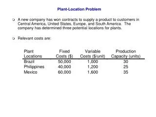
Plant-Location Problem A new company has won contracts to supply a product to customers in Central America, United States, Europe, and South America. The company has determined three potential locations for plants. Relevant costs are:. Customer. Plant. Central America. 9. 30. 18.

E N D
Plant-Location Problem • A new company has won contracts to supply a product to customers in Central America, United States, Europe, and South America. The company has determined three potential locations for plants. • Relevant costs are:
Customer Plant Central America 9 30 18 Brazil 9 7 5 United States 15 7 7 Philippines 25 4 6 Europe 20 3 4 Mexico 7 35 South America 12 9 Plant-Location Problem: Customer Demands and Shipping Costs Numbers on arcs represent shipping costs (in $100 per unit). Which plant location/shipping plan combination minimizes production and distribution costs?
Plant-Location Model • Indices: Let B represent the Brazil plant, and similarly use P (Philippines), M (Mexico), C (Central America), U (United States), E (Europe), and S (South America) • Decision Variables: • Plant opening decisions: and define yPand yMsimilarly. • Production decisions: pB = # of units to produce in Brazil and similarly define pP and pM. • Distribution decisions: xBC = # of units to ship from Brazil to Central America, and define xBU , xBE , …, xMSsimilarly.
Plant-Location Model • Objective Function: Total cost = fixed + variable + shipping costs Total fixed cost: FIX = 50,000 yB + 40,000 yP + 60,000 yM Total variable cost is: VAR = 1,000 pB + 1,200 pP + 1,600 pM . Total shipping cost is: SHIP = 900 xBC + 900 xBU+ 700 xBE+ 500 xBS • + 700 xPC+700 xPU + 400 xPE + 600 xPS • +300 xMC+ 400 xMU+ 700 xME+ 900 xMS .
Plant-Location Model (continued) • Constraints: Plant-production definitions: There are constraints to define total production at each plant. For example, the total production at the Mexico plant is: pM = xMC+ xMU+ xME+ xMS This can be thought of as a “flow in = flow out” constraint for the Mexico node. • Demand constraints: There are constraints to ensure demand is met for each customer. For example, the constraint for Europe is: xBE+ xPE+ xME= 20. This is a “flow in = flow out” constraint for the Europe node. • Plant-Capacity Constraints: Production cannot exceed plant capacity, e.g., for Brazil pB 30
Additional Constraints (continued) • If yB= 0 we want to rule out production at the Brazil plant • If yB= 1, the plant is open and its “available” capacity is 30 units per month • Let’s try this: pB 30 yB If yB= 0 then the constraint becomes pB 0. If yB= 1 then the constraint becomes pB 30. • Alternatively, if pB 0 (and yBcan only take on the values 0 or 1) then yB= 1
Cost definitions: • (VAR Def.) VAR = 1,000 pB + 1,200 pP + 1,600 pM . • (SHIP Def.)SHIP = 900 xBC+ 900 xBU+ 700 xBE+500 xBS • + 700 xPC+700 xPU, + 400 xPE+ 600 xPS • + 300 xMC+ 400 xMU+ 700 xME+ 900 xMS • (FIX Def.) FIX = 50,000 yB + 40,000 yP + 60,000 yM • Plant production definitions: • (Brazil) pB = xBC+ xBU+ xBE+ xBS • (Philippines) pP = xPC+ xPU+ xPE+ xPS • (Mexico) pM = xMC+ xMU+ xME+ xMS • Demand constraints: • (Central America) xBC+ xPC+ xMC = 18 • (United States) xBU+ xPU+ xMU = 15 • (Europe) xBE+ xPE+ xME =20 • (South America) xBS+ xPS+ xMS = 12 • Modified plant capacity constraints: • (Brazil) pB 30 yB • (Philippines) pP 25 yP • (Mexico) pM 35 yM • Binary variables:yB , yP , yM= 0 or 1 • Nonnegativity: All variables 0 Plant Location Integer Programming Model min VAR + SHIP + FIX
The Petromor Bidding Example • Petromor, the national oil company of a small African state, is selling unexploited land with good oil-extraction potential to private oil companies • For each piece of land (or zone, in the oil lingo), Petromor has projected the number of barrels that can potentially be extracted in this zone. • Petromor has organized a public bid in which private oil companies present sealed offers ($ per barrel) for the zones they are interested in buying
The Petromor Bidding Problem • The companies present different bids for different zones. • If a company wins a certain zone, the final price it pays is determined by multiplying the offer in the bid by the zone's potential oil volume, as estimated by the government. • No oil company can be awarded more than one zone as a result of the public offering
The Petromor Bidding Problem • Petromor would like to maximize the revenue resulting from these sales: Table 1. Bids (in $ per Barrel) A B C D E F Zone 1 $8.75 $8.70 $8.80 $8.65 $8.60 $8.50 Zone 2 $6.80 $7.15 $7.25 $7.00 $7.20 $6.85 Zone 3 $8.30 $8.20 $8.70 $7.90 $8.50 $8.40 Zone 4 $7.60 $8.00 $8.10 $8.00 $8.05 $7.85 Table 2. Zone potential (in # of Barrels) Potential Zone 1 205,000 Zone 2 240,000 Zone 3 215,000 Zone 4 225,000 What is the most profitable assignment of zones to the companies in this case?