Download
1 / 21
210 likes | 591 Vues
B1.4 - Derivatives of Primary Trigonometric Functions. IB Math HL/SL - Santowski. We will predict the what the derivative function of f(x) = sin(x) looks like from our curve sketching ideas: We will simply sketch 2 cycles

E N D
B1.4 - Derivatives of Primary Trigonometric Functions IB Math HL/SL - Santowski
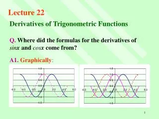
We will predict the what the derivative function of f(x) = sin(x) looks like from our curve sketching ideas: We will simply sketch 2 cycles (i) we see a maximum at /2 and -3 /2 derivative must have x-intercepts (ii) we see intervals of increase on (-2,-3/2), (-/2, /2), (3/2,2) derivative must increase on this intervals (iii) the opposite is true of intervals of decrease (iv) intervals of concave up are (-,0) and ( ,2) so derivative must increase on these domains (v) the opposite is true for intervals of concave up So the derivative function must look like the cosine function!! (A) Derivative of the Sine Function - Graphically
We will predict the what the derivative function of f(x) = sin(x) looks like from our curve sketching ideas: We will simply sketch 2 cycles (i) we see a maximum at /2 and -3 /2 derivative must have x-intercepts (ii) we see intervals of increase on (-2,-3/2), (-/2, /2), (3/2,2) derivative must increase on this intervals (iii) the opposite is true of intervals of decrease (iv) intervals of concave up are (-,0) and ( ,2) so derivative must increase on these domains (v) the opposite is true for intervals of concave up So the derivative function must look like the cosine function!! (A) Derivative of the Sine Function - Graphically
(B) Derivative of Sine Function - Algebraically • We will go back to our limit concepts for determining the derivative of y = sin(x) algebraically
(B) Derivative of Sine Function - Algebraically • So we come across 2 special trigonometric limits: • and • So what do these limits equal? • We will introduce a new theorem called a Squeeze (or sandwich) theorem if we that our limit in question lies between two known values, then we can somehow “squeeze” the value of the limit by adjusting/manipulating our two known values • So our known values will be areas of sectors and triangles sector DCB, triangle ACB, and sector ACB
(C) Applying “Squeeze Theorem” to Trig. Limits • We have sector DCB and sector ACB “squeezing” the triangle ACB • So the area of the triangle ACB should be “squeezed between” the area of the two sectors
(C) Applying “Squeeze Theorem” to Trig. Limits • Working with our area relationships (make h = ) • We can “squeeze or sandwich” our ratio of sin(h) / h between cos(h) and 1/cos(h)
(C) Applying “Squeeze Theorem” to Trig. Limits • Now, let’s apply the squeeze theorem as we take our limits as h 0+ (and since sin(h) has even symmetry, the LHL as h 0- ) • Follow the link to Visual Calculus - Trig Limits of sin(h)/h to see their development of this fundamental trig limit
(C) Applying “Squeeze Theorem” to Trig. Limits • Now what about (cos(h) – 1) / h and its limit we will treat this algebraically
x y -0.05000 0.99958 -0.04167 0.99971 -0.03333 0.99981 -0.02500 0.99990 -0.01667 0.99995 -0.00833 0.99999 0.00000 undefined 0.00833 0.99999 0.01667 0.99995 0.02500 0.99990 0.03333 0.99981 0.04167 0.99971 0.05000 0.99958 (D) Fundamental Trig. Limits Graphic and Numeric Verification
(D) Derivative of Sine Function • Since we have our two fundamental trig limits, we can now go back and algebraically verify our graphic “estimate” of the derivative of the sine function:
(E) Derivative of the Cosine Function • Knowing the derivative of the sine function, we can develop the formula for the cosine function • First, consider the graphic approach as we did previously
We will predict the what the derivative function of f(x) = cos(x) looks like from our curve sketching ideas: We will simply sketch 2 cycles (i) we see a maximum at 0, -2 & 2 derivative must have x-intercepts (ii) we see intervals of increase on (-,0), (, 2) derivative must increase on this intervals (iii) the opposite is true of intervals of decrease (iv) intervals of concave up are (-3/2,-/2) and (/2 ,3/2) so derivative must increase on these domains (v) the opposite is true for intervals of concave up So the derivative function must look like some variation of the sine function!! (E) Derivative of the Cosine Function
We will predict the what the derivative function of f(x) = cos(x) looks like from our curve sketching ideas: We will simply sketch 2 cycles (i) we see a maximum at 0, -2 & 2 derivative must have x-intercepts (ii) we see intervals of increase on (-,0), (, 2) derivative must increase on this intervals (iii) the opposite is true of intervals of decrease (iv) intervals of concave up are (-3/2,-/2) and (/2 ,3/2) so derivative must increase on these domains (v) the opposite is true for intervals of concave up So the derivative function must look like the negative sine function!! (E) Derivative of the Cosine Function
(E) Derivative of the Cosine Function • Let’s set it up algebraically:
So we will go through our curve analysis again f(x) is constantly increasing within its domain f(x) has no max/min points f(x) changes concavity from con down to con up at 0,+ f(x) has asymptotes at +3 /2, +/2 (F) Derivative of the Tangent Function - Graphically
So we will go through our curve analysis again: F(x) is constantly increasing within its domain f `(x) should be positive within its domain F(x) has no max/min points f ‘(x) should not have roots F(x) changes concavity from con down to con up at 0,+ f ‘(x) changes from decrease to increase and will have a min F(x) has asymptotes at +3 /2, +/2 derivative should have asymptotes at the same points (F) Derivative of the Tangent Function - Graphically
(F) Derivative of the Tangent Function - Algebraically • We will use the fact that tan(x) = sin(x)/cos(x) to find the derivative of tan(x)
(G) Internet Links • Calculus I (Math 2413) - Derivatives - Derivatives of Trig Functions from Paul Dawkins • Visual Calculus - Derivative of Trigonometric Functions from UTK • Differentiation of Trigonometry Functions - Online Questions and Solutions from UC Davis • The Derivative of the Sine from IEC - Applet
(H) Homework • Stewart, 1989, Chap 7.2, Q1-5,11