Understanding Query Execution in Database Engines: Concepts and Techniques
This lecture focuses on the essential components of query execution within database engines. It covers key topics including SQL query parsing, the architecture of a database engine, logical and physical query plans, and various optimization strategies. Key operations explored include unions, intersections, and joins, alongside the principles of logical algebra. Practical examples include the creation of logical query plans and the evaluation of physical operators, emphasizing the importance of cost parameters and performance considerations in executing database queries efficiently.

Understanding Query Execution in Database Engines: Concepts and Techniques
E N D
Presentation Transcript
Lecture 23:Query Execution Wednesday, November 23, 2005
Outline • Query execution: 15.1 – 15.5
Architecture of a Database Engine SQL query Parse Query Logicalplan Select Logical Plan Queryoptimization Select Physical Plan Physicalplan Query Execution
Logical Algebra Operators • Union, intersection, difference • Selection s • Projection P • Join |x| • Duplicate elimination d • Grouping g • Sorting t
Logical Query Plan T3(city, c) SELECT city, count(*) FROM sales GROUP BY city HAVING sum(price) > 100 P city, c T2(city,p,c) s p > 100 T1(city,p,c) g city, sum(price)→p, count(*) → c sales(product, city, price) T1, T2, T3 = temporary tables
Logical Query Plan SELECT S.buyer FROM Purchase P, Person Q WHERE P.buyer=Q.name AND Q.city=‘seattle’ AND Q.phone > ‘5430000’ buyer City=‘seattle’ phone>’5430000’ Buyer=name Person Purchase
buyer City=‘seattle’ phone>’5430000’ Buyer=name (Simple Nested Loops) Person Purchase (Table scan) (Index scan) Physical Query Plan SELECT S.buyer FROM Purchase P, Person Q WHERE P.buyer=Q.name AND Q.city=‘seattle’ AND Q.phone > ‘5430000’ • Query Plan: • logical tree • implementation choice at every node • scheduling of operations. Some operators are from relational algebra, and others (e.g., scan) are not.
Question in Class Logical operator: Product(pname, cname) || Company(cname, city) Propose three physical operators for the join, assuming the tables are in main memory:
Question in Class Product(pname, cname) |x| Company(cname, city) • 1000000 products • 1000 companies How much time do the following physical operators take if the data is in main memory ? • Nested loop join time = • Sort and merge = merge-join time = • Hash join time =
Cost Parameters In database systems the data is on disks, not in main memory The cost of an operation = total number of I/Os Cost parameters: • B(R) = number of blocks for relation R • T(R) = number of tuples in relation R • V(R, a) = number of distinct values of attribute a
Cost Parameters • Clustered table R: • Blocks consists only of records from this table • B(R) T(R) / blockSize • Unclustered table R: • Its records are placed on blocks with other tables • When R is unclustered: B(R) T(R) • When a is a key, V(R,a) = T(R) • When a is not a key, V(R,a)
Cost Cost of an operation =number of disk I/Os needed to: • read the operands • compute the result Cost of writing the result to disk is not included on the following slides
Scanning a Table • Clustered relation: • Table scan: • Result may be unsorted: B(R) • Result needs to be sorted: 3B(R) • Index scan • Unsorted: B(R) • Sorted: B(R) or 3B(R) • Unclustered relation • Unsorted: T(R) • Sorted: T(R) + 2B(R)
One-Pass Algorithms Selection s(R), projection P(R) • Both are tuple-at-a-time algorithms • Cost: B(R) Unary operator Input buffer Output buffer
One-pass Algorithms Hash join: R |x| S • Scan S, build buckets in main memory • Then scan R and join • Cost: B(R) + B(S) • Assumption: B(S) <= M
One-pass Algorithms Duplicate elimination d(R) • Need to keep tuples in memory • When new tuple arrives, need to compare it with previously seen tuples • Balanced search tree, or hash table • Cost: B(R) • Assumption: B(d(R)) <= M
Question in Class Grouping: Product(name, department, quantity) gdepartment, sum(quantity) (Product) Answer(department, sum) Question: how do you compute it in main memory ? Answer:
One-pass Algorithms Grouping: g department, sum(quantity) (R) • Need to store all departments in memory • Also store the sum(quantity) for each department • Balanced search tree or hash table • Cost: B(R) • Assumption: number of departments fits in memory
One-pass Algorithms Binary operations: R ∩ S, R ∪ S, R – S • Assumption: min(B(R), B(S)) <= M • Scan one table first, then the next, eliminate duplicates • Cost: B(R)+B(S)
Question in Class What do wedo in each ofthese cases: R ∩ S, R ∪ S, R – S H emptyHashTable/* scan R */ For each x in R do insert(H, x )/* scan S */ For each y in S do _____________________/* collect result */for each z in H do output(z)
Nested Loop Joins • Tuple-based nested loop R ⋈ S • Cost: T(R) B(S) when S is clustered • Cost: T(R) T(S) when S is unclustered for each tuple r in R do for each tuple s in S do if r and s join then output (r,s)
Nested Loop Joins • We can be much more clever • Question: how would you compute the join in the following cases ? What is the cost ? • B(R) = 1000, B(S) = 2, M = 4 • B(R) = 1000, B(S) = 3, M = 4 • B(R) = 1000, B(S) = 6, M = 4
Nested Loop Joins • Block-based Nested Loop Join for each (M-2) blocks bs of S do for each block br of R do for each tuple s in bs for each tuple r in br do if “r and s join” then output(r,s)
. . . Nested Loop Joins Join Result R & S Hash table for block of S (M-2 pages) . . . . . . Output buffer Input buffer for R
Nested Loop Joins • Block-based Nested Loop Join • Cost: • Read S once: cost B(S) • Outer loop runs B(S)/(M-2) times, and each time need to read R: costs B(S)B(R)/(M-2) • Total cost: B(S) + B(S)B(R)/(M-2) • Notice: it is better to iterate over the smaller relation first • R |x| S: R=outer relation, S=inner relation