Adaptive Query Processing
Adaptive Query Processing. Amol Deshpande, University of Maryland Zachary G. Ives, University of Pennsylvania Vijayshankar Raman, IBM Almaden Research Center. Thanks to Joseph M. Hellerstein, University of California, Berkeley. Query Processing: Adapting to the World. d env. d app. <<.

Adaptive Query Processing
E N D
Presentation Transcript
Adaptive Query Processing Amol Deshpande, University of Maryland Zachary G. Ives, University of Pennsylvania Vijayshankar Raman, IBM Almaden Research Center Thanks to Joseph M. Hellerstein, University of California, Berkeley
Query Processing: Adapting to the World denv dapp << dt dt Data independence facilitates modern DBMS technology • Separates specification (“what”) from implementation (“how”) • Optimizer maps declarative query algebraic operations Platforms, conditions are constantly changing: Query processing adapts implementation to runtime conditions • Static applications dynamic environments
Query Optimization and Processing(As Established in System R [SAC+’79]) cardinalitiesindex lo/hi key Dynamic Programming + Pruning Heuristics Professor Course Student > UPDATE STATISTICS ❚ > SELECT * FROM Professor P, Course C, Student S WHERE P.pid = C.pid AND S.sid = C.sid❚
Traditional Optimization Is Breaking denv dt In traditional settings: • Queries over many tables • Unreliability of traditional cost estimation • Success & maturity make problems more apparent, critical In new environments: • e.g. data integration, web services, streams, P2P, sensor nets, hosting • Unknown and dynamic characteristics for data and runtime • Increasingly aggressive sharing of resources and computation • Interactivity in query processing Note two distinct themes lead to the same conclusion: • Unknowns: even static properties often unknown in new environments and often unknowable a priori • Dynamics: can be very high Motivates intra-query adaptivity
A Call for Greater Adaptivity System R adapted query processing as stats were updated • Measurement/analysis: periodic • Planning/actuation: once per query • Improved thru the late 90s (see [Graefe ’93][Chaudhuri ’98]) Better measurement, models, search strategies INGRES adapted execution many times per query • Each tuple could join with relations in a different order • Different plan space, overheads, frequency of adaptivity Didn’t match applications & performance at that time Recent work considers adaptivity in new contexts
Observations on 20thC Systems • Both INGRES & System R used adaptive query processing • To achieve data independence • They “adapt” at different timescales • Ingres goes ‘round the whole loop many times per query • System R decouples parts of loop, and is coarser-grained • measurement/modeling: periodic • planning/actuation: once per query • Query Post-Mortem reveals different relational plan spaces • System R is direct: each query mapped to a single relational algebra stmt • Ingres’ decision space generates a union of plans over horizontal partitions • this “super-plan” not materialized -- recomputed via FindMin • Both have zero-overhead actuation • Never waste query processing work
Tangentially Related Work • An incomplete list!!! • Competitive Optimization [Antoshenkov93] • Choose multiple plans, run in parallel for a time, let the most promising finish • 1x feedback: execution doesn’t affect planning after the competition • Parametric Query Optimization [INSS92, CG94, etc.] • Given partial stats in advance. Do some planning and prune the space. At runtime, given the rest of statistics, quickly finish planning. • Changes interaction of Measure/Model and Planning • No feedback whatsoever, so nothing to adapt to! • “Self-Tuning”/“Autonomic” Optimizers [CR94, CN97, BC02, etc.] • Measure query execution (e.g. cardinalities, etc.) • Enhances measurement, on its own doesn’t change the loop • Consider building non-existent physical access paths (e.g. indexes, partitions) • In some senses a separate loop – adaptive database design • Longer timescales
Tangentially Related Work II • Robust Query Optimization [CHG02, MRS+04, BC05, etc.] • Goals: • Pick plans that remain predictable across wide ranges of scenarios • Pick least expected cost plan • Changes cost function for planning, not necessarily the loop. • If such functions are used in adaptive schemes, less fluctuation [MRS+04] • Hence fewer adaptations, less adaptation overhead • Adaptive query operators [NKT88, KNT89, PCL93a, PCL93b] • E.g. memory-adaptive sort and hash-join • Doesn’t address whole-query optimization problems • However, if used with AQP, can result in complex feedback loops • Especially if their actions affect each other’s models!
Extended Topics in Adaptive QP • An incomplete list!! • Parallelism & Distribution • River [A-D03] • FLuX [SHCF03, SHB04] • Distributed eddies [TD03] • Data Streams • Adaptive load shedding • Shared query processing
Tutorial Focus By necessity, we will cover only a piece of the picture here • Intra-query adaptivity: • autonomic / self-tuning optimization [CR’94, CN’97, BC’02, …] • robust / least expected cost optimization [CHG’02, MRS+’04, BC’05, ...] • parametric or competitive optimization [A’93, INSS’92, CG’94, …] • adaptive operators, e.g., memory adaptive sort & hash join [NKT’88, KNT’89, PCL’93a, PCL’93b,…] • Conventional relations, rather than streams • Single-site, single query computation • For more depth, see our survey in now Publishers’ Foundations and Trends in Databases, Vol. 1 No. 1
Tutorial Outline • Motivation • Non-pipelined execution • Pipelined execution • Selection ordering • Multi-way join queries • Putting it all in context • Recap/open problems
Late Binding; Staged Execution MJ materialization point Materialization points make natural decision points where the next stage can be changed with little cost: • Re-run optimizer at each point to get the next stage • Choose among precomputed set of plans – parametric query optimization [INSS’92, CG’94, …] • Normal execution: pipelines separated by materialization points • e.g., at a sort, GROUP BY, etc. MJ C sort B sort NLJ A R
Mid-query Reoptimization[KD’98,MRS+04] MJ Choose checkpoints at which to monitor cardinalities Balance overhead and opportunities for switching plans If actual cardinality is too different from estimated, Avoid unnecessary plan re-optimization (where the plan doesn’t change) Re-optimize to switch to a new plan Try to maintain previous computation during plan switching • Most widely studied technique: -- Federated systems (InterViso 90, MOOD 96), Red Brick, Query scrambling (96), Mid-query re-optimization (98), Progressive Optimization (04), Proactive Reoptimization (05), … MJ MJ C sort HJ B B sort C NLJ A R Where? When? How? Challenges
Where to Place Checkpoints? MJ Lazy checkpoints: placed above materialization points • No work need be wasted if we switch plans here Eager checkpoints: can be placed anywhere • May have to discard some partially computed results • Useful where optimizer estimates have high uncertainty • More checkpoints more opportunities for switching plans • Overhead of (simple) monitoring is small [SLMK’01] • Consideration: it is easier to switch plans at some checkpoints than others MJ C Lazy sort B sort Eager NLJ A R
When to Re-optimize? • Suppose actual cardinality is different from estimates:how high a difference should trigger a re-optimization? • Idea: do not re-optimize if current plan is still the best • Heuristics-based [KD’98]: e.g., re-optimize < time to finish execution • Validity range[MRS+04]: precomputed range of a parameter (e.g., a cardinality) within which plan is optimal • Place eager checkpoints where the validity range is narrow • Re-optimize if value falls outside this range • Variation: bounding boxes [BBD’05]
How to Reoptimize Getting a better plan: • Plug in actual cardinality information acquired during this query (as possibly histograms), and re-run the optimizer Reusing work when switching to the better plan: • Treat fully computed intermediate results as materialized views • Everything that is under a materialization point • Note: It is optional for the optimizer to use these in the new plan • Other approaches are possible (e.g., query scrambling [UFA’98])
Adapting Pipelined Queries Adapting pipelined execution is often necessary: • Too few materializations in today’s systems • Long-running queries • Wide-area data sources • Potentially endless data streams The tricky issues: • Some results may have been delivered to the user • Ensuring correctness non-trivial • Database operators build up state • Must reason about it during adaptation • May need to manipulate state
Adapting Pipelined Queries We discuss three subclasses of the problem: Selection ordering (stateless) Very good analytical and theoretical results Increasingly important in web querying, streams, sensornets Certain classes of join queries reduce to them Select-project-join queries (stateful) History-independent execution Operator state largely independent of execution history Execution decisions for a tuple independent of prior tuples History-dependent execution Operator state depends on execution history Must reason about the state during adaptation
Adaptive Selection Ordering Complex predicates on single relations common • e.g., on an employee relation: ((salary > 120000) AND (status = 2)) OR ((salary between 90000 and 120000) AND (age < 30) AND (status = 1)) OR … Selection ordering problem: Decide the order in which to evaluate the individual predicates against the tuples We focus on conjunctive predicates(containing only AND’s) Example Query select * from R where R.a = 10 and R.b < 20 and R.c like ‘%name%’;
Basics: Static Optimization R.c like … R.a = 10 R.a = 10 R.b < 20 R.b < 20 R.c like … R R result result Find a single order of the selections to be used for all tuples Query Query plans considered select * from R where R.a = 10 and R.b < 20 and R.c like ‘%name%’; 3! = 6 distinct plans possible
Static Optimization R.c like … R.a = 10 R.b < 20 R result Independence assumption Cost metric: CPU instructions Computing the cost of a plan • Need to know the costsand the selectivitiesof the predicates R1 R2 R3 • costs c1 c2 c3 • selectivities s1 s2 s3 • cost per c1 + s1 c2 + s1 s2 c3 • tuple cost(plan) = |R| * (c1 + s1 * c2 + s1 * s2 * c3)
Static Optimization Rank ordering algorithm for independent selections [IK’84] • Apply the predicates in the decreasing order of rank: (1 – s) / c where s = selectivity, c = cost For correlated selections: • NP-hard under several different formulations • e.g. when given a random sample of the relation • Greedy algorithm, shown to be 4-approximate [BMMNW’04]: • Apply the selection with the highest (1 - s)/c • Compute the selectivities of remaining selections over the result • Conditional selectivities • Repeat Conditional Plans ? [DGHM’05]
Adaptive Greedy [BMMNW’04] R1 R2 R3 R.c like … R.c like … R.a = 10 R.a = 10 R.b < 20 R.b < 20 R result Costs 1 unit 1 unit 1 unit Initial estimated selectivities 0.05 0.1 0.2 Context: Pipelined query plans over streaming data Example: Three independent predicates Optimal execution plan orders by selectivities (because costs are identical)
Adaptive Greedy [BMMNW’04] R1 R2 R3 R.c like … R.a = 10 R.b < 20 R result Profile • Monitor the selectivities over recent past (sliding window) • Re-optimize if the predicates not ordered by selectivities Randomly sample R.a = 10 estimate selectivities of the predicates over the tuples of the profile R.b < 20 Rsample R.c like … Reoptimizer IF the current plan not optimal w.r.t. these new selectivities THEN reoptimize using the Profile
Adaptive Greedy [BMMNW’04] R1 Randomly sample R2 R3 R.c like … R.a = 10 R.b < 20 R result R.a = 10 monitor selectivities sel(R.a = 10), sel(R.b < 20), sel(R.c …) R.b < 20 Rsample (Profile) R.c like … monitor conditional selectivities sel(R.b < 20 | R.a = 10) sel(R.c like … | R.a = 10) sel(R.c like … | R.a = 10 and R.b < 20) Correlated Selections • Must monitor conditional selectivities Reoptimizer Uses conditional selectivities to detect violations Uses the profile to reoptimize O(n2) selectivities need to be monitored
Adaptive Greedy [BMMNW’04] Advantages: • Can adapt very rapidly • Handles correlations • Theoretical guarantees on performance [MBMW’05] Not known for any other AQP algorithms Disadvantages: • May have high runtime overheads • Profile maintenance • Must evaluate a (random) fraction of tuples against all operators • Detecting optimality violations • Reoptimization cost • Can require multiple passes over the profile
Eddies [AH’00] A traditional pipelined query plan R1 R2 R3 R.c like … R.a = 10 R.b < 20 R result R.a = 10 Eddy R.b < 20 R result R.c like … Query processing as routing of tuples through operators Pipelined query execution using an eddy • An eddy operator • Intercepts tuples from sources and output tuples from operators • Executes query by routing source • tuples through operators Encapsulates all aspects of adaptivity in a “standard” dataflow operator: measure, model, plan and actuate.
Eddies [AH’00] R.a = 10 Eddy R.b < 20 R result R.c like … An R Tuple: r1 r1 r1
Eddies [AH’00] Operator 1 ready bit i : 1 operator i can be applied 0 operator i can’t be applied R.a = 10 Operator 2 Eddy R.b < 20 R result R.c like … Operator 3 An R Tuple: r1 r1
Eddies [AH’00] Operator 1 done bit i : 1 operator i has been applied 0 operator i hasn’t been applied R.a = 10 Operator 2 Eddy R.b < 20 R result R.c like … Operator 3 An R Tuple: r1 r1
Eddies [AH’00] Operator 1 R.a = 10 Used to decide validity and need of applying operators Operator 2 Eddy R.b < 20 R result R.c like … Operator 3 An R Tuple: r1 r1
Eddies [AH’00] Operator 1 R.a = 10 Operator 2 Eddy R.b < 20 R result R.c like … Operator 3 An R Tuple: r1 not satisfied For a query with only selections, ready = complement(done) r1 r1 r1 satisfied r1 eddy looks at the next tuple
Eddies [AH’00] Operator 1 satisfied R.a = 10 Operator 2 Eddy R.b < 20 satisfied R result R.c like … Operator 3 satisfied An R Tuple: r2 r2
Eddies [AH’00] Operator 1 satisfied R.a = 10 Operator 2 Eddy R.b < 20 satisfied R result R.c like … Operator 3 satisfied An R Tuple: r2 if done = 111, send to output r2 r2
Eddies [AH’00] Operator 1 R.a = 10 Operator 2 Eddy R.b < 20 R result R.c like … Operator 3 Adapting order is easy • Just change the operators to which tuples are sent • Can be done on a per-tuple basis • Can be done in the middle of tuple’s “pipeline” How are the routing decisions made? Using a routing policy
Routing Policy 1: Non-adaptive table lookups very efficient Operator 1 R.a = 10 Operator 2 Eddy R.b < 20 R result R.c like … Operator 3 • Simulating a single static order • E.g. operator 1, then operator 2, then operator 3 Routing policy: if done = 000 route to 1 100 route to 2 110 route to 3
Overhead of Routing • PostgreSQL implementation of eddies using bitset lookups [Telegraph Project] • Queries with 3 selections, of varying cost • Routing policy uses a single static order, i.e., no adaptation
Routing Policy 2: Deterministic Operator 1 R.a = 10 Operator 2 Eddy R.b < 20 R result R.c like … Operator 3 • Monitor costs and selectivities continuously • Reoptimize periodically using KBZ Can use the A-Greedy policy for correlated predicates Statistics Maintained: Costs of operators Selectivities of operators Routing policy: Use a single order for a batch of tuples Periodically apply KBZ
Overhead of Routing and Reoptimization • Adaptation using batching • Reoptimized every X tuples using monitored selectivities • Identical selectivities throughout experiment measures only the overhead
Routing Policy 3: Lottery Scheduling Operator 1 R.a = 10 Operator 2 Eddy R.b < 20 R result R.c like … Operator 3 • Originally suggested routing policy [AH’00] • Applicable when each operator runs in a separate “thread” • Can also be done single-threaded, via an event-driven query executor • Uses two easily obtainable pieces of information for making routing decisions: • Busy/idle status of operators • Tickets per operator
Routing Policy 3: Lottery Scheduling Rule: IF operator busy, THEN do not route more tuples to it BUSY Operator 1 R.a = 10 Operator 2 Eddy R.b < 20 IDLE R result R.c like … Operator 3 IDLE • Routing decisions based on busy/idle status of operators Rationale: Every thread gets equal time SO IF an operator is busy, THEN its cost is perhaps very high
Routing Policy 3: Lottery Scheduling Operator 1 R.a = 10 Operator 2 Eddy R.b < 20 result R.c like … Operator 3 • Routing decisions based on tickets Rules: 1. Route a new tuple randomly weighted according to the number of tickets tickets(O1) = 10 tickets(O2) = 70 tickets(O3) = 20 Will be routed to: O1 w.p. 0.1 O2 w.p. 0.7 O3 w.p. 0.2 r
Routing Policy 3: Lottery Scheduling Operator 1 R.a = 10 Operator 2 Eddy R.b < 20 result R.c like … Operator 3 • Routing decisions based on tickets Rules: 1. Route a new tuple randomly weighted according to the number of tickets tickets(O1) = 10 tickets(O2) = 70 tickets(O3) = 20 r
Routing Policy 3: Lottery Scheduling Operator 1 R.a = 10 Operator 2 Eddy R.b < 20 result R.c like … Operator 3 • Routing decisions based on tickets Rules: 1. Route a new tuple randomly weighted according to the number of tickets 2. route a tuple to an operator Oi tickets(Oi) ++; tickets(O1) = 11 tickets(O2) = 70 tickets(O3) = 20
Routing Policy 3: Lottery Scheduling Operator 1 R.a = 10 Operator 2 Eddy R.b < 20 result R.c like … Operator 3 • Routing decisions based on tickets Rules: 1. Route a new tuple randomly weighted according to the number of tickets 2. route a tuple to an operator Oi tickets(Oi) ++; 3. Oi returns a tuple to eddy tickets(Oi) --; tickets(O1) = 11 tickets(O2) = 70 tickets(O3) = 20 r
Routing Policy 3: Lottery Scheduling Operator 1 R.a = 10 Operator 2 Eddy R.b < 20 Will be routed to: O2 w.p. 0.777 O3 w.p. 0.222 result R.c like … Operator 3 • Routing decisions based on tickets Rules: 1. Route a new tuple randomly weighted according to the number of tickets 2. route a tuple to an operator Oi tickets(Oi) ++; 3. Oi returns a tuple to eddy tickets(Oi) --; tickets(O1) = 10 tickets(O2) = 70 tickets(O3) = 20 r
Routing Policy 3: Lottery Scheduling Operator 1 R.a = 10 Operator 2 Eddy R.b < 20 result R.c like … Operator 3 • Routing decisions based on tickets Rules: 1. Route a new tuple randomly weighted according to the number of tickets 2. route a tuple to an operator Oi tickets(Oi) ++; 3. Oi returns a tuple to eddy tickets(Oi) --; tickets(O1) = 10 tickets(O2) = 70 tickets(O3) = 20 Rationale: Tickets(Oi) roughly corresponds to (1 - selectivity(Oi)) So more tuples are routed to the more selective operators

