Adaptive Query Processing: Evolution and Modern Practices in Database Optimization
This tutorial revisits adaptive query processing, a foundational concept in database management, tracing its roots back to early systems like System R. It emphasizes the separation of specification and implementation, highlighting the critical role of query optimization in achieving data independence. As environments evolve, traditional optimization methods struggle with dynamic data characteristics and resource sharing. This discourse analyzes modern adaptations, considering new architectures and innovative strategies, ultimately redefining how we approach query processing amidst growing complexities in real-time data environments.

Adaptive Query Processing: Evolution and Modern Practices in Database Optimization
E N D
Presentation Transcript
Adaptive Query Processing Adapted from a Tutorial given at SIGMOD 2006 by: Amol Deshpande, University of Maryland Joseph M. Hellerstein, University of California, Berkeley Vijayshankar Raman, IBM Almaden Research Center
Data Independence Redux dapp denv << dt dt • The taproot of modern database technology • Separation of specification (“what”) from implementation (“how”) • Refamiliarizing ourselves: Why do we care about data independence?
D. I. Adaptivity • Query Optimization: the key to data independence • bridges specification and implementation • isolates static applications from dynamic environments • How does a DBMS account for dynamics in the environment? • This tutorial is on a 30-year-old topic • With a 21st-Century renaissance ADAPTIVITY
Why the Renaissance? ? denv dt • Breakdown of traditional query optimization • Queries over many tables • Unreliability of traditional cost estimation • Success & maturity make problems more apparent, critical • c.f. Oracle v6! • Query processing in new environments • E.g. data integration, web services, streams, P2P, sensornets, hosting, etc. • Unknown and dynamic characteristics for data and runtime • Increasingly aggressive sharing of resources and computation • Interactivity in query processing • Note two separate themes? • Unknowns: even static properties often unknown in new environments • and often unknowable a priori • Dynamics: can be very high -- motivates intra-query adaptivity
20th Century Summary • System R’s optimization scheme deemed the winner for 25 years • Nearly all 20thC research varied System R’s individual steps • More efficient measurement (e.g. sampling) • More efficient/effective models (samples, histograms, sketches) • Expanded plan spaces (new operators, bushy trees, richer queries and data models, materialized views, parallelism, remote data sources, etc) • Alternative planning strategies (heuristic and enumerative) • Speaks to the strength of the scheme • independent innovation on multiple fronts • as compared with tight coupling of INGRES • But… minimal focus on the interrelationship of the steps • Which, as we saw from Ingres, also affects the plan space
21st Century Adaptive Query Processing • (well, starts in late 1990’s) • Revisit basic architecture of System R • In effect, change the basic adaptivity loop! • As you examine schemes, keep an eye on: • Rate of change in the environment that is targeted • How radical the scheme is wrt the System R scheme • ease of evolutionary change • Increase in plan space: are there new, important opportunities? • even if environment is ostensibly static! • New overheads introduced • How amenable the scheme is to independent innovation at each step • Measure/Analyze/Plan/Actuate
Tangentially Related Work • An incomplete list!!! • Competitive Optimization [Antoshenkov93] • Choose multiple plans, run in parallel for a time, let the most promising finish • 1x feedback: execution doesn’t affect planning after the competition • Parametric Query Optimization [INSS92, CG94, etc.] • Given partial stats in advance. Do some planning and prune the space. At runtime, given the rest of statistics, quickly finish planning. • Changes interaction of Measure/Model and Planning • No feedback whatsoever, so nothing to adapt to! • “Self-Tuning”/“Autonomic” Optimizers [CR94, CN97, BC02, etc.] • Measure query execution (e.g. cardinalities, etc.) • Enhances measurement, on its own doesn’t change the loop • Consider building non-existent physical access paths (e.g. indexes, partitions) • In some senses a separate loop – adaptive database design • Longer timescales
Tangentially Related Work II • Robust Query Optimization [CHG02, MRS+04, BC05, etc.] • Goals: • Pick plans that remain predictable across wide ranges of scenarios • Pick least expected cost plan • Changes cost function for planning, not necessarily the loop. • If such functions are used in adaptive schemes, less fluctuation [MRS+04] • Hence fewer adaptations, less adaptation overhead • Adaptive query operators [NKT88, KNT89, PCL93a, PCL93b] • E.g. memory-adaptive sort and hash-join • Doesn’t address whole-query optimization problems • However, if used with AQP, can result in complex feedback loops • Especially if their actions affect each other’s models!
Extended Topics in Adaptive QP • An incomplete list!! • Parallelism & Distribution • River [A-D03] • FLuX [SHCF03, SHB04] • Distributed eddies [TD03] • Data Streams • Adaptive load shedding • Shared query processing
Adaptive Selection Ordering Title slide
Selection Ordering • Complex predicates on relations common • Eg., on an employee relation: ((salary > 120000) AND (status = 2)) OR ((salary between 90000 and 120000) AND (age < 30) AND (status = 1)) OR … • Selection ordering problem Decide the order in which to evaluate the individual predicates against the tuples • We focus on evaluating conjunctive predicates (containing only AND’s) Example Query select * from R where R.a = 10 and R.b < 20 and R.c like ‘%name%’;
Why Study Selection Ordering • Many join queries reduce to this problem • Queries posed against a star schema • Queries where only pipelined left-deep plans are considered • Queries involving web indexes • Increasing interest in recent years • Web indexes [CDY’95, EHJKMW’96, GW’00] • Web services [SMWM’06] • Data streams [AH’00, BMMNW’04] • Sensor Networks [DGMH’05] • Similar to many problems in other domains • Sequential testing (e.g. for fault detection) [SF’01, K’01] • Learning with attribute costs [KKM’05]
Execution Strategies result R • For each tuple r Є R • Apply predicate R.a = 10 first; • If tuple satisfies the selection, apply R.b < 20; • If both satisfied, apply R.c like ‘%name%’; R.c like … R.a = 10 R.b < 20 Pipelined execution (tuple-at-a-time) Static optimization ? 1. Using the KBZ algorithm Order by c/(1-p) Assumes predicate independence 2. A greedy algorithm Known to be 4-approximate
Adaptive Greedy [BMMNW’04] R1 R2 R3 R.c like … R.c like … R.a = 10 R.a = 10 R.b < 20 R.b < 20 R result Costs 1 unit 1 unit 1 unit Initial estimated selectivities 0.05 0.1 0.2 • Context: Pipelined query plans over streaming data • Example: Three independent predicates Optimal execution plan orders by selectivities (because costs are identical)
Adaptive Greedy [BMMNW’04] R1 R2 R3 R.c like … R.a = 10 R.b < 20 R result Profile • Monitor the selectivities • Switch order if the predicates not ordered by selectivities Randomly sample R.a = 10 estimate selectivities of the predicates over the tuples of the profile R.b < 20 Rsample R.c like … Reoptimizer IF the current plan not optimal w.r.t. these new selectivities THEN reoptimize using the Profile
Adaptive Greedy [BMMNW’04] R1 Randomly sample R2 R3 R.c like … R.a = 10 R.b < 20 R result R.a = 10 monitor selectivities sel(R.a = 10), sel(R.b < 20), sel(R.c …) R.b < 20 Rsample (Profile) R.c like … monitor conditional selectivities sel(R.b < 20 | R.a = 10) sel(R.c like … | R.a = 10) sel(R.c like … | R.a = 10 and R.b < 20) • Correlated Selections • Must monitor conditional selectivities Reoptimizer Uses conditional selectivities to detect violations Uses the profile to reoptimize O(n2) selectivities need to be monitored
Adaptive Greedy [BMMNW’04] • Advantages: • Can adapt very rapidly • Theoretical guarantees on performance • Not known for any other AQP protocols • Disadvantages: • Limited applicability • Only applies to selection ordering and specific types of join queries • Possibly high runtime overheads • Several heuristics described in the paper
Eddies [AH’00] A traditional pipelined query plan R1 R2 R3 R.c like … R.a = 10 R.b < 20 R result R.a = 10 Eddy R.b < 20 R result R.c like … • Treat query processing as routing of tuples through operators Pipelined query execution using an eddy • An eddy operator • Intercepts tuples from sources and output tuples from operators • Executes query by routing source • tuples through operators
Eddies [AH’00] R.a = 10 Eddy R.b < 20 R result R.c like … An R Tuple: r1 r1 r1
Eddies [AH’00] Operator 1 ready bit i : 1 operator i can be applied 0 operator i can’t be applied R.a = 10 Operator 2 Eddy R.b < 20 R result R.c like … Operator 3 An R Tuple: r1 r1
Eddies [AH’00] Operator 1 done bit i : 1 operator i has been applied 0 operator i hasn’t been applied R.a = 10 Operator 2 Eddy R.b < 20 R result R.c like … Operator 3 An R Tuple: r1 r1
Eddies [AH’00] Operator 1 R.a = 10 Used to decide validity and need of applying operators Operator 2 Eddy R.b < 20 R result R.c like … Operator 3 An R Tuple: r1 r1
Eddies [AH’00] Operator 1 R.a = 10 Operator 2 Eddy R.b < 20 R result R.c like … Operator 3 An R Tuple: r1 not satisfied For a query with only selections, ready = complement(done) r1 r1 r1 satisfied r1 eddy looks at the next tuple
Eddies [AH’00] Operator 1 satisfied R.a = 10 Operator 2 Eddy R.b < 20 satisfied R result R.c like … Operator 3 satisfied An R Tuple: r2 r2
Eddies [AH’00] Operator 1 satisfied R.a = 10 Operator 2 Eddy R.b < 20 satisfied R result R.c like … Operator 3 satisfied An R Tuple: r2 if done = 111, send to output r2 r2
Eddies [AH’00] Operator 1 R.a = 10 Operator 2 Eddy R.b < 20 R result R.c like … Operator 3 • Adapting order is easy • Just change the operators to which tuples are sent • Can be done on a per-tuple basis • Can be done in the middle of tuple’s “pipeline” • How are the routing decisions made ? • Using a routing policy
Routing Policy 1: Non-adaptive table lookups very efficient Operator 1 R.a = 10 Operator 2 Eddy R.b < 20 R result R.c like … Operator 3 • Simulating a single static order • E.g. operator 1, then operator 2, then operator 3 Routing policy: if done = 000 route to 1 100 route to 2 110 route to 3
Overhead of Routing • PostgreSQL implementation of eddies using bitset lookups [Telegraph Project] • Queries with 3 selections, of varying cost • Routing policy uses a single static order, i.e., no adaptation
Routing Policy 2: Deterministic Operator 1 R.a = 10 Operator 2 Eddy R.b < 20 R result R.c like … Operator 3 • Monitor costs and selectivities continuously • Reoptimize periodically using KBZ Can use the A-Greedy policy for correlated predicates Statistics Maintained: Costs of operators Selectivities of operators Routing policy: Use a single order for a batch of tuples Periodically apply KBZ
Overhead of Routing and Reoptimization • Adaptation using batching • Reoptimized every X tuples using monitored selectivities • Identical selectivities throughout experiment measures only the overhead
Routing Policy 3: Lottery Scheduling Operator 1 R.a = 10 Operator 2 Eddy R.b < 20 R result R.c like … Operator 3 • Originally suggested routing policy [AH’00] • Applicable when each operator runs in a separate “thread” • Can also be done single-threaded, via an event-driven query executor • Uses two easily obtainable pieces of information for making routing decisions: • Busy/idle status of operators • Tickets per operator
Routing Policy 3: Lottery Scheduling Rule: IF operator busy, THEN do not route more tuples to it BUSY Operator 1 R.a = 10 Operator 2 Eddy R.b < 20 IDLE R result R.c like … Operator 3 IDLE • Routing decisions based on busy/idle status of operators Rationale: Every thread gets equal time SO IF an operator is busy, THEN its cost is perhaps very high
Routing Policy 3: Lottery Scheduling Operator 1 R.a = 10 Operator 2 Eddy R.b < 20 result R.c like … Operator 3 • Routing decisions based on tickets Rules: 1. Route a new tuple randomly weighted according to the number of tickets tickets(O1) = 10 tickets(O2) = 70 tickets(O3) = 20 Will be routed to: O1 w.p. 0.1 O2 w.p. 0.7 O3 w.p. 0.2 r
Routing Policy 3: Lottery Scheduling Operator 1 R.a = 10 Operator 2 Eddy R.b < 20 result R.c like … Operator 3 • Routing decisions based on tickets Rules: 1. Route a new tuple randomly weighted according to the number of tickets tickets(O1) = 10 tickets(O2) = 70 tickets(O3) = 20 r
Routing Policy 3: Lottery Scheduling Operator 1 R.a = 10 Operator 2 Eddy R.b < 20 result R.c like … Operator 3 • Routing decisions based on tickets Rules: 1. Route a new tuple randomly weighted according to the number of tickets 2. route a tuple to an operator Oi tickets(Oi) ++; tickets(O1) = 11 tickets(O2) = 70 tickets(O3) = 20
Routing Policy 3: Lottery Scheduling Operator 1 R.a = 10 Operator 2 Eddy R.b < 20 result R.c like … Operator 3 • Routing decisions based on tickets Rules: 1. Route a new tuple randomly weighted according to the number of tickets 2. route a tuple to an operator Oi tickets(Oi) ++; 3. Oi returns a tuple to eddy tickets(Oi) --; tickets(O1) = 11 tickets(O2) = 70 tickets(O3) = 20 r
Routing Policy 3: Lottery Scheduling Operator 1 R.a = 10 Operator 2 Eddy R.b < 20 Will be routed to: O2 w.p. 0.777 O3 w.p. 0.222 result R.c like … Operator 3 • Routing decisions based on tickets Rules: 1. Route a new tuple randomly weighted according to the number of tickets 2. route a tuple to an operator Oi tickets(Oi) ++; 3. Oi returns a tuple to eddy tickets(Oi) --; tickets(O1) = 10 tickets(O2) = 70 tickets(O3) = 20 r
Routing Policy 3: Lottery Scheduling Operator 1 R.a = 10 Operator 2 Eddy R.b < 20 result R.c like … Operator 3 • Routing decisions based on tickets Rules: 1. Route a new tuple randomly weighted according to the number of tickets 2. route a tuple to an operator Oi tickets(Oi) ++; 3. Oi returns a tuple to eddy tickets(Oi) --; tickets(O1) = 10 tickets(O2) = 70 tickets(O3) = 20 Rationale: Tickets(Oi) roughly corresponds to (1 - selectivity(Oi)) So more tuples are routed to the more selective operators
Routing Policy 3: Lottery Scheduling • Effect of the combined lottery scheduling policy: • Low cost operators get more tuples • Highly selective operators get more tuples • Some tuples are randomly, knowingly routed according to sub-optimal orders • To explore • Necessary to detect selectivity changes over time
Routing Policy 4: Content-based Routing Operator 1 Eddy result Operator 2 • Routing decisions made based on the values of the attributes [BBDW’05] • Also called “conditional planning” in a static setting [DGHM’05] • Less useful unless the predicates are expensive • At the least, more expensive than r.d > 100 Expensive predicates Example Eddy notices: R.d > 100 sel(op1) > sel(op2) & R.d < 100 sel(op1) < sel(op2) Routing decisions for new tuple “r”: IF (r.d > 100): Route to op1 first w.h.p ELSE Route to op2 first w.h.p
Eddies: Post-Mortem • Cost of adaptivity • Routing overheads • Minimal with careful engineering • E.g. using bitset-indexed routing arrays • “Batching” helps tremendously • Statistics Maintenance • Executing the routing policy logic
Discussion • Benefits for AQP techniques come from two places • Increased explored plan space • Can use different plans for different parts of data • Adaptation • Can change the plan according to changing data characteristics • Selection ordering is STATELESS • No inherent “cost of switching plans” • Can switch the plan without worrying about operator states • Key to the simplicity of the techniques
Discussion • Adaptation is not free • Costs of monitoring and maintaining statistics can be very high • A selection operation may take only 1 instruction to execute • Comparable to updating a count • “Sufficient statistics” • May need to maintain only a small set of statistics to detect violations • E.g. The O(n2) matrix in Adaptive-Greedy [BBMNW’04]
Adaptive Join Processing Title slide
Outline • 20th Century Adaptivity: Intuition from the Classical Systems • Adaptive Selection Ordering • Adaptive Join Processing • Additional complexities beyond selection ordering • Four plan spaces • Simplest: pipelines of Nested Loop Joins • Traditional: Trees of Binary Operators (TOBO) • Multi-TOBO: horizontal partitioning • Dataflows of unary operators • Handling asynchrony • Research Roundup
Select-Project-Join Processing SMJ NLJ T S R • Query: select count(*) from R, S, T where R.a=S.aandS.b=T.b and S.c like ‘%name%’ and T.d = 10 • An execution plan • Cost metric: CPU + I/O • Plan Space: • Traditionally, tree of binary join operators (TOBO): • access methods • Join algorithms • Join order • Adaptive systems: • Some use the same plan space, but switch between plans during execution • Others use much larger plan spaces • different adaptation techniques adapt within different plan spaces
Approach NLJ NLJ NLJ B C A • Pipelined nested-loops plans • Static Rank Ordering • Dynamic Rank Ordering – Eddies, Competition • Trees of Binary Join Operators (TOBO) • Static: System R • Dynamic: Switching plans during execution Multiple Trees of Binary Join Operators • Convergent Query Processing • Eddies with Binary Join Operators • STAIRs: Moving state across joins • Dataflows of Unary Operators • N-way joinsswitching join algorithms during execution • Asynchrony in Query Processing
Pipelined Nested Loops Join R NLJ NLJ NLJ B C A • Simplest method of joining tables • Pick a driver table (R). Call the rest driven tables • Pick access methods (AMs) on the driven tables • Order the driven tables • Flow R tuples through the driven tables For each r R do:look for matches for r in A;for each match a do: look for matches for <r,a> in B; …
Adapting a Pipelined Nested Loops Join NLJ NLJ NLJ B C A Almost identical to selection ordering • Simplest method of joining tables • Pick a driver table (R). Call the rest driven tables • Pick access methods (AMs) on the driven tables • Order the driven tables • Flow R tuples through the driven tables For each r R do:look for matches for r in A;for each match a do: look for matches for <r,a> in B; … R Keep this fixed for now
Tree Of Binary Join Operators (TOBO) recap • Standard plan space considered by most DBMSs today • Pick access methods, join order, join algorithms • search in this plan space done by dynamic programming NLJ MJ HJ C D NLJ B A R

