Download

1 / 60
610 likes | 700 Vues
Explore imperfect representations and observations of the world, the impact of laziness and efficiency on decision-making, and models of uncertainty in AI. Learn about non-deterministic and probabilistic approaches to handling uncertainty in agents. Discover the significance of belief states and probabilistic distributions in dealing with uncertainty. |

E N D
3 Sources of Uncertainty • Imperfect representations of the world • Imperfect observation of the world • Laziness, efficiency
On(A,B) On(B,Table) On(C,Table) Clear(A) Clear(C) A A A B C B C B C First Source of Uncertainty:Imperfect Predictions • There are many more states of the real world than can be expressed in the representation language • So, any state represented in the language may correspond to many different states of the real world, which the agent can’t represent distinguishably • The language may lead to incorrect predictions about future states
Real world in some state Interpretation of the percepts in the representation language Percepts On(A,B) On(B,Table) Handempty Observation of the Real World Percepts can be user’s inputs, sensory data (e.g., image pixels), information received from other agents, ...
R1 R2 Second source of Uncertainty:Imperfect Observation of the World • Observation of the world can be: • Partial, e.g., a vision sensor can’t see through obstacles (lack of percepts) The robot may not know whether there is dust in room R2
A B C Second source of Uncertainty:Imperfect Observation of the World • Observation of the world can be: • Partial, e.g., a vision sensor can’t see through obstacles • Ambiguous, e.g., percepts have multiple possible interpretations On(A,B) On(A,C)
Second source of Uncertainty:Imperfect Observation of the World • Observation of the world can be: • Partial, e.g., a vision sensor can’t see through obstacles • Ambiguous, e.g., percepts have multiple possible interpretations • Incorrect
Third Source of Uncertainty:Laziness, Efficiency • An action may have a long list of preconditions, e.g.: Drive-Car: P = Have-Keys Empty-Gas-Tank Battery-Ok Ignition-Ok Flat-Tires Stolen-Car ... • The agent’s designer may ignore some preconditions ... or by laziness or for efficiency, may not want to include all of them in the action representation • The result is a representation that is either incorrect – executing the action may not have the described effects – or that describes several alternative effects
Representation of Uncertainty • Many models of uncertainty • We will consider two important models: • Non-deterministic model:Uncertainty is represented by a set of possible values, e.g., a set of possible worlds, a set of possible effects, ... • Probabilistic (stochastic) model:Uncertainty is represented by a probabilistic distribution over a set of possible values
0.2 0.3 0.4 0.1 Example: Belief State • In the presence of non-deterministic sensory uncertainty, an agent belief state represents all the states of the world that it thinks are possible at a given time or at a given stage of reasoning • In the probabilistic model of uncertainty, a probability is associated with each state to measure its likelihood to be the actual state
This state would occur 20% of the times 0.2 0.3 0.4 0.1 What do probabilities mean? • Probabilities have a natural frequency interpretation • The agent believes that if it was able to return many times to a situation where it has the same belief state, then the actual states in this situation would occur at a relative frequency defined by the probabilistic distribution
Cavity Cavity p 1-p Example • Consider a world where a dentist agent D meets a new patient P • D is interested in only one thing: whether P has a cavity, which D models using the proposition Cavity • Before making any observation, D’s belief state is: • This means that D believes that a fraction p of patients have cavities
Cavity Cavity p 1-p Example • Probabilities summarize the amount of uncertainty (from our incomplete representations, ignorance, and laziness)
Non-deterministic vs. Probabilistic • Non-deterministic uncertainty must always consider the worst case, no matter how low the probability • Reasoning with sets of possible worlds • “The patient may have a cavity, or may not” • Probabilistic uncertainty considers the average case outcome, so outcomes with very low probability should not affect decisions (as much) • Reasoning with distributions of possible worlds • “The patient has a cavity with probability p”
Non-Deterministic vs. Probabilistic • If the world is adversarial and the agent uses probabilistic methods, it is likely to fail consistently(unless the agent has a good idea of how the world thinks, see Texas Hold-em) • If the world is non-adversarial and failure must be absolutely avoided, then non-deterministic techniques are likely to be more efficient computationally • In other cases, probabilistic methods may be a better option, especially if there are several “goal” states providing different rewards and life does not end when one is reached
Other Approaches to Uncertainty • Fuzzy Logic • Truth value of continuous quantities interpolated from 0 to 1 (e.g., X is tall) • Problems with correlations • Dempster-Shafer theory • Bel(X) probability that observed evidence supports X • Bel(X) 1-Bel(X) • Optimal decision making not clear under D-S theory
Probabilistic Belief • Consider a world where a dentist agent D meets with a new patient P • D is interested in only whether P has a cavity; so, a state is described with a single proposition – Cavity • Before observing P, D does not know if P has a cavity, but from years of practice, he believes Cavity with some probability p and Cavity with probability 1-p • The proposition is now a booleanrandom variable and (Cavity, p) is a probabilistic belief
An Aside • The patient either has a cavity or does not, there is no uncertainty in the world. What gives? • Probabilities are assessed relative to the agent’s state of knowledge • Probability provides a way of summarizing the uncertainty that comes from ignorance or laziness • “Given all that I know, the patient has a cavity with probability p” • This assessment might be erroneous (given an infinite number of patients, the true fraction may be q ≠ p) • The assessment may change over time as new knowledge is acquired (e.g., by looking in the patient’s mouth)
Where do probabilities come from? • Frequencies observed in the past, e.g., by the agent, its designer, or others • Symmetries, e.g.: • If I roll a dice, each of the 6 outcomes has probability 1/6 • Subjectivism, e.g.: • If I drive on Highway 37 at 75mph, I will get a speeding ticket with probability 0.6 • Principle of indifference: If there is no knowledge to consider one possibility more probable than another, give them the same probability
Multivariate Belief State • We now represent the world of the dentist D using three propositions – Cavity, Toothache, and PCatch • D’s belief state consists of 23 = 8 states each with some probability: {CavityToothachePCatch,CavityToothachePCatch, CavityToothachePCatch,...}
The belief state is defined by the full joint probability of the propositions Probability table representation
Probabilistic Inference P(Cavity Toothache) = 0.108 + 0.012 + ... = 0.28
Probabilistic Inference P(Cavity) = 0.108 + 0.012 + ... = 0.2
Probabilistic Inference Marginalization:P(C) = StSpP(Ctp) using the conventions that C = Cavity or Cavity and that St is the sum over t = {Toothache, Toothache}
Probabilistic Inference Marginalization:P(C) = StSpP(Ctp) using the conventions that C = Cavity or Cavity and that St is the sum over t = {Toothache, Toothache}
Probabilistic Inference P(CavityPCatch) = 0.016 + 0.144 = 0.16
Probabilistic Inference Marginalization:P(CP) = StP(CtP) using the conventions that C = Cavity or Cavity, P = PCatchor PCatchand that St is the sum over t = {Toothache, Toothache}
Possible Worlds Interpretation • A probability distribution associates a number to each possible world • If is the set of possible worlds, and is a possible world, then a probability model P() has • 0 P() 1 • P()=1 • Worlds may specify all past and future events
Events (Propositions) • Something possibly true of a world (e.g., the patient has a cavity, the die will roll a 6, etc.) expressed as a logical statement • Each event e is true in a subset of • The probability of an event is defined as • P(e) = P() I[e is true in ] • Where I[x] is the indicator function that is 1 if x is true and 0 otherwise
Komolgorov’s Probability Axioms • 0 P(a) 1 • P(true) = 1, P(false) = 0 • P(a b) = P(a) + P(b) - P(a b) • Hold for all events a, b • HenceP(a) = 1-P(a)
Conditional Probability • P(a|b) is the posterior probability of a given knowledge that event b is true • “Given that I know b, what do I believe about a?” • P(a|b) = /b P() I[a is true in ] • Where /b is the set of worlds in which b is true • P(|b): A probability distribution over a restricted set of worlds! • If a new piece of information c arrives, the agent’s new belief (if it obeys the rules of probability) should beP(a|bc)
Conditional Probability • P(ab) = P(a|b) P(b) = P(b|a) P(a)P(a|b) is the posterior probability of a given knowledge of b • Axiomatic definition: P(a|b) = P(ab)/P(b)
Conditional Probability • P(ab) = P(a|b) P(b) = P(b|a) P(a) • P(abc) = P(a|bc) P(bc) = P(a|bc) P(b|c) P(c) • P(Cavity) = StSp P(Cavitytp) = StSpP(Cavity|tp) P(tp) = StSpP(Cavity|tp) P(t|p) P(p)
Probabilistic Inference P(Cavity|Toothache) = P(CavityToothache)/P(Toothache) = (0.108+0.012)/(0.108+0.012+0.016+0.064) = 0.6 Interpretation: After observing Toothache, the patient is no longer an “average” one, and the prior probability (0.2) of Cavity is no longer valid P(Cavity|Toothache) is calculated by keeping the ratios of the probabilities of the 4 cases of Toothache unchanged, and normalizing their sum to 1
Independence • Two events a and b are independent if P(a b) = P(a) P(b) hence P(a|b) = P(a) • Knowing bdoesn’t give you any information about a
Conditional Independence • Two events a and b are conditionally independent given c, if P(a b|c) = P(a|c) P(b|c)hence P(a|b,c) = P(a|c) • Once you know c, learning b doesn’t give you any information about a
Random Variables • In a possible world, a random variable X can take on one of a set of values Val(X)={x1,…,xn} • Such an event is written ‘X=x’ • Capital: random variable • Lowercase: assignment of variable to value • Truth assignments to boolean random variables may also be expressed as ‘X’ or ‘X’
Notation with Random Variables • Capital letters A,B,C denote random variables • Each random variable X can take one of a set of possible values xVal(X) • Boolean random variable has Val(X)={True,False} • Although the most unambiguous way of writing a probabilistic belief is over an event… • P(X=x) = a number • P(X=x Y=y) = a number • …it is tedious to list a large number of statements that hold for multiple values x and y • Random variables allow using a shorthand notation (unfortunately a source of a lot of initial confusion!)
Decoding Probability Notation • Mental rule #1: Lowercase: assignments are often left implicit when unambiguous • P(a) = P(A=a) = a number
Decoding Probability Notation (Boolean variables) • P(X=True) is written P(X) • P(X=False) is written P(X) • [Since P(X) = 1-P(X), knowing P(X) is enough to specify the whole distribution over X=True or X=False]
Decoding Probability Notation • Mental rule #2: Drop the AND, use commas • P(a,b) = P(ab) = P(A=aB=b) = a number
Decoding Probability Notation • Mental rule #3: Uppercase => values left implicit • Suppose Val(X) = {1,2,3} • When I write P(X), it states “the distribution defined over all of P(X=1), P(X=2), P(X=3)” • It is not a single number, but rather a set of numbers • P(X) = [A probability table]
Decoding Probability Notation • P(A,B) = [P(A=a B=b) for all combinations of aVal(A), bVal(B)] • A probability table with |Val(A)|x|Val(B)| entries
Decoding Probability Notation • Mental rule #3: Uppercase => values left implicit • So when you see f(A,B)=g(A,B) this means: • “f(a,b) = g(a,b) for all values of aVal(A) and bVal(B)” • f(A,B)=g(A) means: • “f(a,b) = g(a) for all values of aVal(A) and bVal(B)” • f(A,b)=g(A,b) means: • “f(a,b) = g(a,b) for all values of aVal(A)” • Order doesn’t matter. P(A,B) is equivalent to P(B,A)
Another Mnemonic: Functional Equalities • P(X) is treated as a function over a variable X • Operations and relations are on “function objects” • If you say f(x) = g(x) without a value of x, then you can infer f(x) = g(x) holds for all x • Likewise if you say f(x,y) = g(x) without stating a value of x or y, then you can infer f(x,y) = g(x) holds for all x,y
Quiz: What does this mean? • P(AB) = P(A)+P(B)- P(AB) • P(A=a B=b) = P(A=a) + P(B=b) • P(A=a B=b) • For all aVal(A) and bVal(B)
Marginalization • If X, Y are boolean random variables that describe the state of the world, then • This generalizes to multiple variables • ++ • Etc.