Recap from last time: live variables

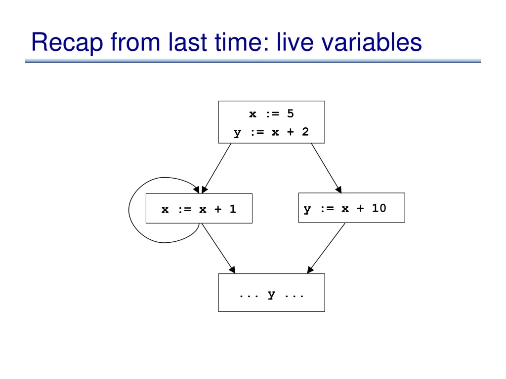
1. Recap from last time: live variables x := 5 y := x + 2 y := x + 10 x := x + 1 ... y ...

2. Revisiting assignment in Fx := y op z(out) = out – { x } [ { y, z} x := y op z out

3. Theory of backward analyses • Can formalize backward analyses in two ways • Option 1: reverse flow graph, and then run forward problem • Option 2: re-develop the theory, but in the backward direction

4. Precision • Going back to constant prop, in what cases would we lose precision?

5. Precision • Going back to constant prop, in what cases would we lose precision? if (...) { x := -1; } else x := 1; } y := x * x; ... y ... if (p) { x := 5; } else x := 4; } ... if (p) { y := x + 1 } else { y := x + 2 } ... y ... x := 5 if (<expr>) { x := 6 } ... x ... where <expr> is equiv to false

6. Precision • The first problem: Unreachable code • solution: run unreachable code removal before • the unreachable code removal analysis will do its best, but may not remove all unreachable code • The other two problems are path-sensitivity issues • Branch correlations: some paths are infeasible • Path merging: can lead to loss of precision

7. MOP: meet over all paths • Information computed at a given point is the meet of the information computed by each path to the program point if (...) { x := -1; } else x := 1; } y := x * x; ... y ...

8. MOP • For a path p, which is a sequence of statements [s1, ..., sn] , define: Fp(in) = Fsn( ...Fs1(in) ... ) • In other words: Fp = • Given an edge e, let paths-to(e) be the (possibly infinite) set of paths that lead to e • Given an edge e, MOP(e) = • For us, should be called JOP...

9. MOP vs. dataflow • As we saw in our example, in general,MOP  dataflow • In what cases is MOP the same as dataflow? Dataflow MOP x := -1; y := x * x; ... y ... x := 1; y := x * x; ... y ... x := -1; x := 1; Merge y := x * x; ... y ... Merge

10. MOP vs. dataflow • As we saw in our example, in general,MOP  dataflow • In what cases is MOP the same as dataflow? • Distributive problems. A problem is distributive if: 8 a, b . F(a t b) = F(a) t F(b)

11. Summary of precision • Dataflow is the basic algorithm • To basic dataflow, we can add path-separation • Get MOP, which is same as dataflow for distributive problems • Variety of research efforts to get closer to MOP for non-distributive problems • To basic dataflow, we can add path-pruning • Get branch correlation • To basic dataflow, can add both: • meet over all feasible paths

12. Program Representations

13. Representing programs • Goals

14. Representing programs • Primary goals • analysis is easy and effective • just a few cases to handle • directly link related things • transformations are easy to perform • general, across input languages and target machines • Additional goals • compact in memory • easy to translate to and from • tracks info from source through to binary, for source-level debugging, profilling, typed binaries • extensible (new opts, targets, language features) • displayable

15. Option 1: high-level syntax based IR • Represent source-level structures and expressions directly • Example: Abstract Syntax Tree

16. Translate input programs into low-level primitive chunks, often close to the target machine Examples: assembly code, virtual machine code (e.g. stack machines), three-address code, register-transfer language (RTL) Standard RTL instrs: Option 2: low-level IR

17. Option 2: low-level IR

18. Comparison

19. Comparison • Advantages of high-level rep • analysis can exploit high-level knowledge of constructs • easy to map to source code (debugging, profiling) • Advantages of low-level rep • can do low-level, machine specific reasoning • can be language-independent • Can mix multiple reps in the same compiler

20. Components of representation • Control dependencies: sequencing of operations • evaluation of if & then • side-effects of statements occur in right order • Data dependencies: flow of definitions from defs to uses • operands computed before operations • Ideal: represent just those dependencies that matter • dependencies constrain transformations • fewest dependences ) flexibility in implementation

21. Control dependencies • Option 1: high-level representation • control implicit in semantics of AST nodes • Option 2: control flow graph (CFG) • nodes are individual instructions • edges represent control flow between instructions • Options 2b: CFG with basic blocks • basic block: sequence of instructions that don’t have any branches, and that have a single entry point • BB can make analysis more efficient: compute flow functions for an entire BB before start of analysis

22. Control dependencies • CFG does not capture loops very well • Some fancier options include: • the Control Dependence Graph • the Program Dependence Graph • More on this later. Let’s first look at data dependencies

23. Data dependencies • Simplest way to represent data dependencies: def/use chains

24. Def/use chains • Directly captures dataflow • works well for things like constant prop • But... • Ignores control flow • misses some opt opportunities since conservatively considers all paths • not executable by itself (for example, need to keep CFG around) • not appropriate for code motion transformations • Must update after each transformation • Space consuming

25. SSA • Static Single Assignment • invariant: each use of a variable has only one def

27. SSA • Create a new variable for each def • Insert  pseudo-assignments at merge points • Adjust uses to refer to appropriate new names • Question: how can one figure out where to insert  nodes using a liveness analysis and a reaching defns analysis.

28. Converting back from SSA • Semantics of x3 := (x1, x2) • set x3 to xi if execution came from ith predecessor • How to implement  nodes?

29. Converting back from SSA • Semantics of x3 := (x1, x2) • set x3 to xi if execution came from ith predecessor • How to implement  nodes? • Insert assignment x3 := x1 along 1st predecessor • Insert assignment x3 := x2 along 2nd predecessor • If register allocator assigns x1, x2 and x3 to the same register, these moves can be removed • x1 .. xn usually have non-overlapping lifetimes, so this is kind of register assignment is legal

30. Common Sub-expression Elim • Want to compute when an expression is available in a var • Domain:

31. Flow functions in FX := Y op Z(in) = X := Y op Z out in FX := Y(in) = X := Y out

32. Flow functions in FX := Y op Z(in) = in – { X ! * } – { * ! ... X ... } [ { X ! Y op Z | X  Y Æ X  Z} X := Y op Z out in FX := Y(in) = in – { X ! * } – { * ! ... X ... } [ { X ! E | Y ! E 2 in } X := Y out

33. Example

34. Example

35. Problems • z := j * 4 is not optimized to z := x, even though x contains the value j * 4 • m := b + a is not optimized, even though a + b was already computed • w := 4 * m it not optimized to w := x, even though x contains the value 4 *m

36. Problems: more abstractly • Available expressions overly sensitive to name choices, operand orderings, renamings, assignments • Use SSA: distinct values have distinct names • Do copy prop before running available exprs • Adopt canonical form for commutative ops

37. Example in SSA in FX := Y op Z(in) = X := Y op Z out in0 in1 FX := Y(in0, in1) = X := (Y,Z) out

38. Example in SSA in X := Y op Z FX := Y op Z(in) = in [ { X ! Y op Z } out in0 in1 FX := Y(in0, in1) = (in0Å in1 ) [ { X ! E | Y ! E 2 in0Æ Z ! E 2 in1 } X := (Y,Z) out

39. Example in SSA

40. Example in SSA

41. What about pointers?

42. What about pointers? • Option 1: don’t use SSA for point-to memory • Option 2: insert copies between SSA vars and real vars

43. SSA helps us with CSE • Let’s see what else SSA can help us with • Loop-invariant code motion

44. Loop-invariant code motion • Two steps: analysis and transformations • Step1: find invariant computations in loop • invariant: computes same result each time evaluated • Step 2: move them outside loop • to top if used within loop: code hoisting • to bottom if used after loop: code sinking