Download
1 / 49
500 likes | 687 Vues
High Resolution Velocity A nalysis for Resource P lays. Bo Zhang and J. T. Kwiatkowski. Outline. Factors that affect the fidelity of velocity analysis High resolution velocity spectrum The engine for a utomatic velocity optimization

E N D
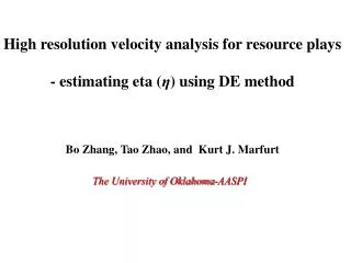
High Resolution Velocity Analysis for Resource Plays Bo Zhang and J. T. Kwiatkowski
Outline • Factors that affect the fidelity of velocity analysis • High resolution velocity spectrum • The engine for automatic velocity optimization • Automatic interval velocity analysis based on DE (workflow) • Synthetic and Real data examples • Conclusion • Road-ahead
Factors that affect the fidelity of velocity analysis Velocity (ft/s) Velocity (ft/s) 1000 1000 12000 12000 14000 14000 0.0 • The resolution of velocity spectrum. 0.5 Time (s) 1.0 Vs. 1.5 Semblance SN based on PFA
Factors that affect the fidelity of velocity analysis • Manually picking velocity at CDP location? • Manually picking velocity for each reflection events? Conventional velocity analysis Dense velocity analysis (http://www.slb.com/services/westerngeco/services/dp/technologies/time/technology/dva.aspx)
Outline • Factors that affect the fidelity of velocity analysis • High resolution velocity spectrum • The engine for automatic velocity optimization • Automatic interval velocity analysis based on DE (workflow) • Synthetic and Real data examples • Conclusion • Road-ahead
High resolution velocity spectrum The seismic trace d(t) can be written as where d(t) is the seismic traces, s(t) is the reflection signal, and n(t) is the noise. Suppose we have M traces in one CDP gather, then Construction the correlation matrix between each traces d_corr
High resolution velocity spectrum Assume the noise and reflected signals are uncorrelated, then the eigenstructure of d_corr has the following properties: • d_corr is not sensitive to amplitude variation (AVO) • In the ideal case, d_corris a rank 1 matrix. • The maximum eigenvalue of d_corris corresponding major underline factors which is regards as the reflected signals. Those two properties suggest giving an estimated signal-to-noise ratio (S/N) to the corrected gather
High resolution velocity spectrum Offset (ft) 0 3000 6000 9000 0.0 0.5 Time (s) 1.0 1.5 Synthetic gather with random noise added
High resolution velocity spectrum Velocity (ft/s) 10000 12000 14000 0.0 0.5 Time (s) 1.0 1.5 semblance
High resolution velocity spectrum Velocity (ft/s) 10000 12000 14000 0.0 0.5 Time (s) 1.0 1.5 SN based on PCA
Outline • Factors that affect the fidelity of velocity analysis • High resolution velocity spectrum • The engine for automatic velocity optimization • Automatic interval velocity analysis based on DE (workflow) • Synthetic and Real data examples • Conclusion • Road-ahead
The engine for automatic velocity optimization Differential evolutionary (DE) algorithm is an efficient and simple global optimization scheme. The basic features can be summarized as follows: Initialization Mutation Crossover Selection DE workflow
The engine for automatic velocity optimization Problem statement and notation • Suppose we want to optimize a function with D real parameters • We must select the size of the population N (it must be at least 4) • The parameter vectors have the form: where G is the generation number.
The engine for automatic velocity optimization • Define upper and lower bounds for each parameter: Initialization • Randomly select initial parameter values uniformly between the upper and lower bounds. Mutation Crossover Selection
The engine for automatic velocity optimization • Each of the N parameter vectors undergoes mutation, recombination and selection • Mutation expands the search space • For a given parameter vector xi,G randomly select the three different vectors: Initialization Mutation Crossover Selection
The engine for automatic velocity optimization • Add the weighted difference of two of the vectors to the third to form the donor vector: Initialization • The mutation factor F is a user defined constant from [0, 2] Mutation Crossover Selection
The engine for automatic velocity optimization • Crossover incorporates successful solutions from the previous generation • The trial vector ui,G+1 is developed from the elements of the target vector, xi,G, and the elements of the donor vector, vi,G+1 • Elements of the donor vector enter the trial vector with probability CR Initialization Mutation Crossover Selection
The engine for automatic velocity optimization if or if or Initialization Mutation , Irandomis a random integer from [1,2,…D] Crossover Selection
The engine for automatic velocity optimization if otherwise Initialization Mutation , Irandomis a random integer from [1,2,…D] Crossover • Mutation, crossover and selection continue until some stopping criterion is reached Selection
Outline • Factors that affect the fidelity of velocity analysis • High resolution velocity spectrum • The engine for automatic velocity optimization • Automatic interval velocity analysis based on DE (workflow) • Synthetic and Real data examples • Conclusion • Road-ahead
Automatic interval velocity analysis Prestack time migrated gather after reverse NMO Conventional migration velocity analysis on the coarse grid Define the analysis time grids along t0 axis for each CDP Initialize the population set based on the conventional velocity model Get the trail interval velocity set by DE operation Compare the semblance value of trail and target interval model. The one with greater semblance value survives into next generation Yes More generations No Output the best member
Outline • Factors that affect the fidelity of velocity analysis • High resolution velocity spectrum • The engine for automatic velocity optimization • Automatic interval velocity analysis based on DE (workflow) • Synthetic and Real data examples • Conclusion • Road-ahead
Synthetic data examples Time (s)
Synthetic data examples Offset (ft) 0 3000 6000 9000 0.0 0.5 Time (s) 1.0 1.5 Synthetic gather
Synthetic data examples Velocity (ft/s) 10000 12000 14000 0.0 0.5 Time (s) 1.0 1.5 semblance
Synthetic data examples Velocity (ft/s) 10000 12000 14000 0.0 0.5 Time (s) 1.0 1.5 SN based PCA
Synthetic data examples Offset (ft) 0 3000 6000 9000 0.0 0.5 Time (s) 1.0 1.5 NMO correction based velocity model from DE
Synthetic data examples Offset (ft) 0 3000 6000 9000 0.0 0.5 Time (s) 1.0 1.5 NMO correction based manual picking velocity model
Synthetic data examples Offset (ft) 0 3000 6000 9000 0.0 0.5 Time (s) 1.0 1.5 Synthetic gather with random noise added
Synthetic data examples Velocity (ft/s) 10000 12000 14000 0.0 0.5 Time (s) 1.0 1.5 semblance
Synthetic data examples Velocity (ft/s) 10000 12000 14000 0.0 0.5 Time (s) 1.0 1.5 SN based PCA
Synthetic data examples Offset (ft) 0 3000 6000 9000 0.0 0.5 Time (s) 1.0 1.5 NMO correction based velocity model from DE
Synthetic data examples Offset (ft) 0 3000 6000 9000 0.0 0.5 Time (s) 1.0 1.5 NMO correction based manual picking velocity model
Real data examples Location map of the Chicontepecforedeep in East-Central Mexico(Sarkar, 2011)
Real data examples high CMP number 1 50 100 0.0 0.5 low Time (s) 1.0 1.5 2.0 Interval velocity from Dix inversion based on RMS velocity
Real data examples high CMP number 1 50 100 0.0 0.5 low Time (s) 1.0 1.5 2.0 Interval velocity based on de search
Real data examples high CMP number 1 50 100 0.0 0.5 low Time (s) 1.0 1.5 2.0 Manually picking RMS velocity
Real data examples high CMP number 1 50 100 0.0 0.5 low Time (s) 1.0 1.5 2.0 RMS velocity from DE optimization
Real data examples CMP number 1 50 100 0.0 0.5 Time (s) 1.0 1.5 2.0 stacked section based on the RMS velocity from manual picking
Real data examples CMP number 1 50 100 0.0 0.5 Time (s) 1.0 1.5 2.0 stacked section based on the RMS velocity from DE optimization
Real data examples high CMP number 1 50 100 0.0 0.5 low Time (s) 1.0 1.5 2.0 Model based Impedance inversion
Outline • Factors that affect the fidelity of velocity analysis • High resolution velocity spectrum • The engine for automatic velocity optimization • Automatic interval velocity analysis based on DE (workflow) • Synthetic and Real data examples • Conclusion • Road-ahead
Conclusion • Interval velocity from RMS velocity strongly suffers the errors contained in the RMS velocity model • From the synthetic testing, interval velocity model from DE optimization is superior to that generated from RMS velocity. • In the real case study, the optimized interval velocity model has more detail than that inverted from RMS velocity • By employing Gardner’s equation, high resolution interval velocity model can be used for model based impedance inversion • Multiples will strongly damage the the optimized interval velocity
Road-ahead • Consider the analysis time location on the section instead of each CDP alone. • Integrate the interpreted horizons into the analysis. • Testing on other surveys.
Acknowledgements • PEMEX for permission to use and show their data • The industry sponsors of the University of Oklahoma Attribute-Assisted Seismic Processing and Interpretation (AASPI) Consortium.