Download

1 / 24
240 likes | 386 Vues
Sediment Land Calibration and Delivery Factor Calculation. Land-River Connection. Edge of Field. BMP factor. Edge of Stream. Land Acre Factor. Delivery Factor. Content. Edge of Field (EOF) calibration Delivery Factor Calculation . = KSER * RO * (RO + Water Storage). J1. Wash off.

E N D
Sediment Land Calibration and Delivery Factor Calculation Chesapeake Bay Program Modeling
Land-River Connection Edge of Field BMP factor Edge of Stream Land Acre Factor Delivery Factor Chesapeake Bay Program Modeling
Content • Edge of Field (EOF) calibration • Delivery Factor Calculation Chesapeake Bay Program Modeling
= KSER * RO * (RO + Water Storage) J1 Wash off Input Attachment Detachment J2 = (1-cover) * KRER* (Rain) Land Sediment Simulation Detached Sediment = NVSI lb/day = AFFIX * (Detached sediment) Soil Matrix (unlimited) Chesapeake Bay Program Modeling
Land Calibration • Calibrate Edge of Field to RUSLE supplied by NRI • Split into major land uses Chesapeake Bay Program Modeling
Group 1 - Forest Harvested Forest Natural grass Extractive Barren Pervious Urban Impervious Urban water Group 2 - Pasture Hay High till with manure High till without manure Low till with manure 13 Land use categories for sediment: Chesapeake Bay Program Modeling
For Each Land Use in group 1: • Mean EOF for entire watershed reach to target - Keep land parameters same everywhere - Use different energy in hydrological processes to drive the difference • Reasons: - Only ONE EOF value available - Avoid over-parameterization Chesapeake Bay Program Modeling
For Each Land Use in group 2: • EOF targets available at county level • Reach EOF county by county • Different land parameters Chesapeake Bay Program Modeling
Attachment Decision Rules for Four Key land Parameters: • Rule1 – 90% detached sed re-attached to soil matrix in 30 days AFFIX = 0.7673 Detached Sediment = AFFIX * (Detached sediment) Chesapeake Bay Program Modeling
Input Detached Sediment • Rule2 – Vertical Input high enough for hysteresis NVSI (lb/acre/day)= a * target load (lb/acre/yr) Assumed a =0.5 for hvf grs pur … NVSI 0.93 9.32 4.11 3.01 … = NVSI lb/day Chesapeake Bay Program Modeling
Rule 3 - Zero Detached Sed after Large Storms Adjust KRER and KSER -No build-up after most big storms - Reach to NRI targets Chesapeake Bay Program Modeling
Forest – 0.34 tons/acre/year Mean = 0.339 Chesapeake Bay Program Modeling
Harvested Forest – 3.4 tons/acre/year Mean = 3.39 Chesapeake Bay Program Modeling
Natural Grass – 1.5 tons/acre/year Mean = 1.498 Chesapeake Bay Program Modeling
Pervious Urban –1.1 tons/acre/year Mean = 1.105 Chesapeake Bay Program Modeling
Land-River Connection Edge of Field BMP factor Edge of Stream Land Acre Factor Delivery Factor Chesapeake Bay Program Modeling
Ideal delivery factor • Vary by segment • Vary by land use type • Vary by flow condition • Last two are like a finer segmentation scheme Chesapeake Bay Program Modeling
Delivery factor methodsEPA region 4 sediment tool • DF = (1 - 0.97 * L / C) ( sun and Mcnulty 1998) • DF = exp(-0.4233*L*exp (-16.1* (Y/L + 0.057)) - 0.6) (Yagow 1988) • DF = 0.417762 * A -0.134958 - 0.127097 (SCS 1983) • DF = .9004 - .1341 (lnL) - .0465 (lnL)2 +.00749 (lnL)3 - .0399 (lnY) +.0144 (lnY)2 +.00308(lnY)3 (Swift 2000) Chesapeake Bay Program Modeling
SCS method Adopted • Similar to successful phase 4 method • Less data intensive and more stable that other methods • Not particular to a land use type • DF = 0.417762 * A -0.134958 - 0.127097 Chesapeake Bay Program Modeling
Proposed method: Relate delivery to average distance from land to river by segment Chesapeake Bay Program Modeling
Single factor for each land use in each segment • Related to watershed size • Unique for each Land use • Assume mean distance is the radius of a circle A = π*(mean distance)^2 Chesapeake Bay Program Modeling
Some Preliminary Results - Chesapeake Bay Program Modeling
Next Step… • Finish EOF calibration • Get ready for river calibration Chesapeake Bay Program Modeling