Download
1 / 24
240 likes | 322 Vues
Transition to turbulence and turbulent bifurcation in a von Karman flow. F.Daviaud SPEC, CEA/Saclay, France In collaboration with A. Chiffaudel, B. Dubrulle, L. Marié, F. Ravelet, P. Cortet. VKS team. Turbulent von Karman flow. Axisymmetry R π symmetry / radial axis R c =100 mm

E N D
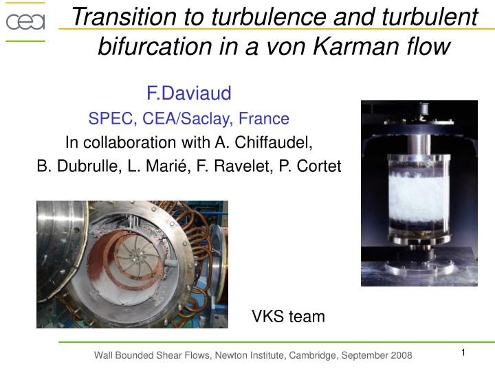
Transition to turbulence and turbulent bifurcation in a von Karman flow F.Daviaud SPEC, CEA/Saclay, France In collaboration with A. Chiffaudel, B. Dubrulle, L. Marié, F. Ravelet, P. Cortet VKS team
Turbulent von Karman flow • Axisymmetry • Rπ symmetry / radial axis • Rc=100 mm • H = 180 mm • f = 2-20 Hz • Re = 2π Rc f2 / ν= 102 – 106 • fluid: water and glycerol-water f1 - + Inertial stirring TM60 propellers Velocity regulation f2
3 « scales » Mean on60 s 500 f -1 Mean on 1/20 s 1/2 f -1 Mean on : 1/500 s 1/50 f -1
First bifurcations and symmetry breaking meridian plane: poloïdal recirculation Re = 90 Stationary axisymmetric Re = 185 m = 2 ; stationary Re = 400 m = 2 ; periodic Tangent plane : shear layer
Time spectra as a function of Re 0.2 0.1 220 225 230 Re = 330 Re = 380 Re = 440 Periodic Quasi-Periodic Chaotic
Time spectra as a function of Re Re = 1000 Re = 4000 2000 < Re < 6500 Chaotic Turbulent Bimodal distribution : signature of the turbulent shear
Transition to turbulence: Azimuthal kinetic energy fluctuations Developed turbulence Globally supercritical transition via a Kelvin-Helmholtz type instability of the shear layer and secondary bifurcations Ravelet et al. JFM 2008 Rec= 330 Ret = 3300
Multiplicity of solutions Kp= Torque/ρRc5 (2π f)2 Rec= 330 Ret = 3300 Re-1
Turbulent Bifurcation of the mean flow Symmetry broken: 2 different mean flows exchange stability. Bifurcated flow (b) : no more shear layer broken symmetry Re = 3.105 two cells one state one cell two states
Turbulent Bifurcation • Kp = Torque/ρRc5 (2π f)2 ΔKp= Kp1- Kp2 • θ = (f2-f1) / (f2+f1) • Re = (f1+f2)1/2 Re = 3.105 Ravelet et al. PRL 2004
Stability of the symmetric state Statistics on 500 runs for different θ • Cumulative distribution • functions of bifurcation time tbif: • P(tbif>t)=A exp(-(t-t0)/τ) • t0f ~ 5 • τ : characteristic bif. time
Stability of the symmetric state • symmetric state • marginally stable • τ→ ∞ when θ→ 0 exponent = -6
Forbidden zone with velocity regulation Forbidden zone for stationary regimes g = (Kp1-Kp2)/(Kp1+Kp2) 1 cell (velocity) 2 cells (velocity) θ = (F1-F2)/(F1+F2)
Forbidden zone with torque regulation (b2) Intermittent states (i) g = (Kp1-Kp2)/(Kp1+Kp2) (s) intermittent states (i) 1 cell (velocity) 1 cell (torque) 2 cells (torque) (b1) θ = (F1-F2)/(F1+F2)
Torque regulation: stochastic transitions 1cell state → 2 cells states Kp1 Kp21 cell Kp1 ~ Kp2, “intermittence” between 2 states q , f Kp1 Kp2 2 cells
VKS dynamo experiment Propellers TM73 Small curvature, diameter 3/4 Meridional annulus
Position of the shear layer = f(θ) -1 -0.5 0 0.5 1 SPIV measurements θc = 0.09 without annulus ◦r = 0.7 Position z of the separatrix ● stagnation point θc = 0.175 with annulus θ = 0.05, without annulus θ = (F1-F2)/(F1+F2) The annulus stabilizes the separatrix
Transition 1 cell - 2 cells at θc= ± 0.175 • quasi-continuous transition • small hysteresis • small Kp difference • very different from TM60 propellers <Kp> <ΔKp> = <Kp1> - <Kp2> θ = (F1-F2)/(F1+F2)
10 min. acquisitions ○ : θ increasing ● : θ decreasing State (b) <ΔKp> State (s) Transition at θc= ± 0.175 Mean ΔKp is continuous Time (sec.) (s) (b) (s)… … (b) … θ = (F1-F2)/(F1+F2) stochastic transition 1 →2 cells Time (sec.)
Transition at θc= ± 0.175 <ΔKp> θ = (F1-F2)/(F1+F2) Measurements : 2 – 200 min
Transition at θc Probability of presence p(s), p(b) θ = (F1-F2)/(F1+F2) θc= 0.174 p(s)/p(b) Cf. de la Torre & Burguete PRL 2007 and Friday talk θ = (F1-F2)/(F1+F2)
Origin of erratic field reversals observed in VKS experiment? θ= 0.17
Bifurcations in turbulent flows: theory? • von Karman : turbulent bifurcation • VKS: dynamo action • and B reversals • 3. Couette flows: turbulent stripes and spirals Prigent, Dauchot et al. PRL 2002