Download
1 / 31
330 likes | 623 Vues
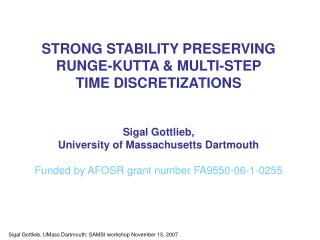
STRONG STABILITY PRESERVING RUNGE-KUTTA & MULTI-STEP TIME DISCRETIZATIONS Sigal Gottlieb, University of Massachusetts Dartmouth Funded by AFOSR grant number FA9550-06-1-0255. My Collaborators:. David Ketcheson University of Washington A student of Randy LeVeque. Colin Macdonald

E N D
STRONG STABILITY PRESERVING RUNGE-KUTTA & MULTI-STEP TIME DISCRETIZATIONS Sigal Gottlieb, University of Massachusetts Dartmouth Funded by AFOSR grant number FA9550-06-1-0255
My Collaborators: David Ketcheson University of Washington A student of Randy LeVeque Colin Macdonald Simon Fraser University, A student of Steven Ruuth
What are strong stability preserving schemes and why do we need them? Strong stability preserving (SSP) high order time discretizations were developed for the time evolution of hyperbolic partial differential equations with discontinuous solutions. Significant effort is expended in creating spatial discretizations which satisfy certain nonlinear stability properties, or non-oscillatory properties, usually when coupled with forward Euler. e.g. Total variation diminishing spatial discretizations, Harten’s lemma.
Spatial discretization of hyperbolicartial differential equations We begin with a hyperbolic partial differential equation If this PDE has a continuous solution, we can use any finite difference, finite-element or spectral method to approximate the spatial derivative, and use the regular (linear) stability analysis to make sure it is stable, and so convergent. However, if the solution is discontinuous, then this stability analysis is not sufficient! In that case, we try to build spatial discretizations which satisfy some nonlinear stability properties when coupled with forward Euler, under some time-step restriction. These methods include total variation diminishing (TVD) and total variation bounded (TVB) schemes, or the essentially non-oscillatory (ENO) or Weighted ENO schemes.
What are strong stability preserving schemes and why do we need them? But Euler’s method is only first order, and we want higher order time discretizations. So the problem is: how do you make sure that the nonlinear stability properties your spatial discretization satisfies when coupled with forward Euler will still be satisfied when the spatial discretization is coupled with a higher order time discretizations? Does this really matter? Consider the following numerical example:
A Numerical Example • Consider the linear advection equation with a square wave initial condition. In this example, we use a simple upwinding spatial discretization, which is unconditionally total variation diminishing with the implicit Euler method. • Although the Crank-Nicolson method is unconditionally linearly stable, it has a time-step limit for nonlinear stability (SSP). • Even when coupled with a total variation diminishing first order spatial discretization, the numerical solution will develop oscillations indicating instability for a sufficiently large time-step. • Note that any spatial discretization that is strongly stable for forward Euler under some time-step restriction is unconditionally stable for backward Euler. Why is this example for implicit methods? The concept is the same, but the numerical results are more dramatic!
A Numerical Example Numerical solution in blueExact solution in red Left: The Crank-Nicolson method has a time-step limit for SSP -- when coupled with a TVD first order spatial discretization, the numerical solution will develop oscillations indicating instability for a sufficiently large time-step. Right: An unconditionally SSP time discretization: No oscillations form.
A nonlinear example of violating the SSP condition Numerical solution in blueExact solution in red Burgers’ equation.
How an oscillation forms . . . As the time-step restriction is exceeded
What are strong stability preserving schemes and why do we need them? These numerical simulations underscore the need for time-discretizations which preserve the strong stability properties of forward Euler. SSP methods give you a guarantee of provable strong stability in any norm, semi-norm or convex functional, as long as the spatial discretization had this property for forward Euler. If you start with a spatial discretization which coupled with forward Euler satisfies certain strong stability properties, under some time-step restriction, then the spatial discretization when coupled with an SSP high order time discretization will still satisfy these strong stability properties, perhaps under a different time-step restriction.
Why does this work? where the operator is strongly stable under forward Euler time-stepping Starting with the ODE under the time step restriction the Runge-Kutta method can be written as a convex combination of forward Euler steps.
Why does this work? This is also true of a multistep method So that these methods produce a solution that is also strongly stable under the modified time step restriction
What’s the catch? The time step restriction can be a problem. Let’s look at some of the popular methods: The second order, two stage method:
An optimal third order method The third order, three stage method:
Some basic results for explicit SSP Runge Kutta methods • For second order and third order, the optimal time step restriction is the same as forward Euler Proof by S. Gottlieb and C.-W. Shu in 1992 • For four-stage fourth order, we need to introduce an adjoint operator, or add a stage, because of the presence of negative coefficients Proof by S. Gottlieb and C.-W. Shu in 1992 • Any method above fourth order will have negative coefficients S. Ruuth and R. Spiteri in 2001
Four stage fourth order method A four-stage fourth order method must have negative coefficients. This poses a problem – because now we no longer have convex combinations of forward Euler, This can be fixed by introducing a “downwinding” operator, which is strongly stable under forward Euler with a negative time-step:
Five stage fourth order method Has CFL coefficient c= 1.508, or an effective CFL coefficient 0.302, which makes it almost as efficient as the third order method, but higher order.
Optimal SSP explicit Runge Kutta methods David Ketcheson just completed a study of explicit low storage SSP Runge-Kutta methods with multiple stages: The observed SSP coefficient in some numerical experiments matches well with the predicted values:
Some interesting connections . . . • Work by Higueras, Ferracina and Spijker 2002 gave us a new view on SSP methods: • There are significant connections between the time step restriction for SSP methods, contractivity, and the radius of absolute monotonicity. • This theory has allowed an efficient algorithm for numerical search among the class of implicit and explicit SSP Runge-Kutta methods
Implicit SSP methods • We expect a time-step restriction for explicit methods, but want to make it as large as possible or to avoid it if at all possible. • We turn to implicit methods in the hope that these will allow us to avoid a time step restriction. • However, this is not the case. The connections to contractivity theory tell us that all Runge-Kutta and multi-step methods of order greater than one will have a step-size restriction. • The question is then: how large can the step-size be, and is this enough to outweigh the extra cost of solving a nonlinear system?
Implicit SSP Runge Kutta methods Using numerical optimization we search for implicit SSP method with optimal time-step restrictions: • Methods of order p=2, 3, 4 of up to 11 stages were found • The second and third order methods are singly diagonally implicit • The fourth order methods are all diagonally implicit • Numerical optimization software was also used to search among methods of order 5 and 6. In this case, the number of coefficients and constraints was much larger and this was a more difficult problem. However, here too all the optimal methods found were diagonally implicit. CONJECTURE: All optimal SSP implicit Runge Kutta methods are diagonally implicit.
Optimal Implicit Runge-Kutta fourth order methods are diagonally implicit • Comparison of DIRK and SDIRK methods:
Optimal Implicit Runge-Kutta fifth order methods are diagonally implicit
Results • Using connections to contractivity theory we can conclude that: The maximum order for implicit methods is 6 and there is a restriction on the stage order • Numerical optimization software used to find methods with largest allowable timestep among all implicit Runge-Kutta methods • Methods of order p=2, 3, 4 of up to 11 stages were found • The second and third order methods are SDIRK • The fourth order methods are all DIRK • Numerical optimization software was also used to search among methods of order 5 and 6. In this case, the number of coefficients and constraints was much larger and this was a more difficult problem. However, here too all the optimal methods found were DIRK.
Conclusions • Explicit SSP Runge-Kutta methods exist for orders up to 4 and stages up to 26 • Explicit SSP multistep methods are given up to 5th order and 6 steps • Complete analysis of SSP implicit Runge-Kutta methods up to order 6 and 11 stages • No SSP IRK of order > 6 • These optimal SSPIRK methods are efficient because they are SDIRK or DIRK and have a sparse structure • What about multi-step methods? There we have the restriction that c=2, even for implicit methods
Publications & Awards • C. Macdonald, S. Gottlieb, and S.J. Ruuth, “A numerical study of diagonally split Runge Kutta methods for PDEs with discontinuities”. • D. Ketcheson, C. Macdonald, S. Gottlieb, “Optimal implicit strong stability preserving Runge-Kutta methods”. • D. Ketcheson, “Highly efficient strong stability preserving Runge-Kutta methods with Low-Storage Implementations”.