Download
1 / 21
210 likes | 354 Vues
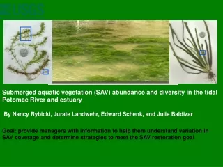
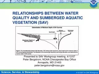
RELATIONSHIPS BETWEEN WATER QUALITY AND SUMBERGED AQUATIC VEGETATION (SAV). Presented to SAV Workgroup meeting, 4/12/07 Peter Bergstrom, NOAA Chesapeake Bay Office Annapolis, MD 21403 peter.bergstrom@noaa.gov. SAV – water clarity relationship.

E N D
RELATIONSHIPS BETWEEN WATER QUALITY AND SUMBERGED AQUATIC VEGETATION (SAV) Presented to SAV Workgroup meeting, 4/12/07 Peter Bergstrom, NOAA Chesapeake Bay Office Annapolis, MD 21403 peter.bergstrom@noaa.gov 4/12/2007 for SAV Workgroup
SAV – water clarity relationship • In general, we expect more SAV to grow in shallow tidal waters where there is better water clarity. • This analysis was done to reexamine this expectation, using recent data and some different tools than those we used in SAV Tech Synthesis I (1992) and II (2000). 4/12/2007 for SAV Workgroup
Main hypotheses examined & conclusions • Weak version: • Segments with better water clarity should have more SAV area, and vice versa • This looks for a generally positive correlation without regard to goal or target attainment • Strong version: • Most of the segments that met the SAV area goal also met the water clarity target, and vice versa • This looks for both positive correlations, and agreement of target or goal attainment • Conclusion: • The data examined supported the weak version, especially in higher salinity segments, but not the strong version. 4/12/2007 for SAV Workgroup
Two additional factors examined - 1 • I used designated use depths in calculating PLW (Percent Light through the Water) for some analyses • A restoration depth (Z) for SAV must be chosen when setting a water clarity habitat requirement, to set how much light needs to reach what depth (at MLLW). Z appears in the exponent in PLW = e –KD*Z. • The concept of variable restoration depths was in SAV Technical Synthesis I in 1992. Most of the Secchi targets assumed this depth was 1 m, as deep as SAV grows in many areas, but there were separate “2 m restoration targets” (rarely used) • Effects of variable restoration depths were explored more fully in Chapter VII of SAV Tech Synthesis II in 2000, using depths of 0, 0.25, 0.5, 1, and 2 m in analyses, but the depth did not vary by segment. 4/12/2007 for SAV Workgroup
Two additional factors examined - 2 • The designated use depths range from 0.5 to 2 m, and were set by CBP segment by MD & VA in 2003 based on the historical distribution of SAV in that segment. • The effect of designated use depths on the attainment of PLW targets has apparently not been examined. They are not currently used in assessing attainment as far as I know. • I also examined attainment of different water clarity targets, including • those adopted in 2000 for SAV growth (PLW > 22% and 13% in high and low salinity), called “old targets” and • those from more recent phytoplankton research, called “new targets.” They range from 11-48% for the 4 salinity regimes, or PLW > 45% and 15% averaged over high and low salinity segments. 4/12/2007 for SAV Workgroup
Analysis approach - 1 • Relationships between two continuous variables (median water clarity and mapped SAV area) are sometimes assessed using scatter plots and correlations, but these approaches do not work well for these data, for a variety of reasons. (see next slide) • Instead I converted each of the continuous variables into 5 categories using ranges that had roughly equal sample sizes in each category, used them on the X-axis, and plotted the distribution of the other (still continuous) variable in those categories on the Y-axis using box plots. Also used Kruskal-Wallis ANOVA on the same data. • Approach was suggested by Claire Buchanan and based on analyses she did relating attainment of phytoplankton goals to attainment of water quality goals. 4/12/2007 for SAV Workgroup
Scatter plots of SAV area vs. water clarity, even when done separately for HI and LO salinity as they were here, simply have too much scatter to be useful. Box plots allow you to see patterns in one continuous variable while the other is binned into categories. In choosing the categories, I tried to equalize the sample size in each category, since box plots based on small sample sizes are not as useful. In the box plots, box width is proportional to sample size (most box plots are not graphed this way). Why I used box plots rather than scatter plots 4/12/2007 for SAV Workgroup
Analysis approach - 2 • I made box plots with both variables on the X-axis (in separate analyses) because while in general, better water clarity allows SAV to grow better, it is also true that large and dense SAV beds can improve water clarity at nearby monitoring stations. • Thus, which variable is cause and which is effect is not entirely clear, so I used each variable in both roles. • The categories were chosen separately for low & high salinity segments, and for PLW_Secchi and PLW_DU clarity variables since their distribution was quite different. • The expected positive monotonic relationship was that the medians for the “y” variable would go up with each increasing “x” category (weak version), and that those medians would exceed the y-axis target (for PLW or SAV area) only in the highest “x” categories (strong version). 4/12/2007 for SAV Workgroup
Caveats about the analysis • It used mid-channel water quality data only, collected once or twice a month. That is the only baywide water quality data set we have. • It uses annual SAV growing season medians of those water quality data, to compare to the single annual SAV area values, both calculated by CBP segment. • It expressed SAV area as a percentage of CBP restoration goals. Since these goals may not show the closest relationship with water clarity, I plan to redo the analysis expressing SAV area as a percentage of the potential habitat (Tier II goal, the area to 1 m restoration depth). • Thus it should be considered a preliminary analysis. I hope that some of its suggested findings can be tested further using nearshore continuous monitoring data over smaller spatial scales. 4/12/2007 for SAV Workgroup
Results – 1 (ANOVA and box plots) • Kruskal-Wallis ANOVA results (did the y variable vary among the x categories?), 8 analyses: • For PLW_Secchi, all 4 of the ANOVA results were significant (P < 0.0004). • For PLW_DU, the ANOVA results were only significant for 3 of the 4 analyses (P < 0.014). They were not significant for HI salinity using categories of PLW_DU (P = 0.16). • Box plot results (8 plots) • There were some different patterns by salinity group using PLW_Secchi (HI salinity had better fit), and • the patterns for PLW_DU (used as the category or the response variable) generally showed a worse fit with expected results than the same graphs for PLW_Secchi. 4/12/2007 for SAV Workgroup
Results – 2: Summary table Table 5. Summary of box plot and ANOVA analyses for HI and LO salinity, using both PLW_Secchi and PLW_DU as the water clarity variables. 4/12/2007 for SAV Workgroup
Results - 3: HI salinity, PLW_Secchi (Z = 1) Both were considered “Good fit” (monotonic increasing) In all plots, box width is proportional to sample size Note tiny 5th category (N=1) 4/12/2007 for SAV Workgroup
Results - 4: LO salinity, PLW_Secchi (Z = 1) Both were considered “Moderate fit” (increasing but not monotonic) 4/12/2007 for SAV Workgroup
Results - 5: HI salinity, PLW_DU (Z = 0.5, 1, or 2) ANOVA was NS (P=0.14) Both were considered “Poor fit,” 1st flat,2nd is V-shaped Note tiny 5th category (N=1) 4/12/2007 for SAV Workgroup
Results – 6: LO salinity, PLW_DU (Z = 0.5, 1, or 2) Were considered “Poor” and “Moderate” fit, 1st is V-shaped 4/12/2007 for SAV Workgroup
Conclusions - 1 • Results supported the weaker version of the expected positive relationship between water clarity and SAV area, especially for high salinity segments • Results did not support the stronger version of this relationship, because the segments that met the water clarity targets often differed from the segments that met the SAV goals. • In high salinity segments, many segments that met the old water clarity target (PLW > 22%) did not meet the SAV goal, while in low salinity segments, many segments that met the SAV goal did not meet the old water clarity target (PLW > 13%). • These discrepancies suggest that the existing high salinity PLW target (22%) may be too low, and the low salinity PLW target (13%) may be too high, to accurately predict SAV growth. However, the low salinity relationships are not very strong. (see below) 4/12/2007 for SAV Workgroup
Conclusions - 2 • Should we start using designated use depths to calculate PLW? No. • Since the box plot patterns for high salinity changed from what we expected (upward trend) to what we did not expect (flat or V-shaped pattern), these analyses do NOT support using designated use depths in water clarity calculations • This conclusion does NOT require any change to the status quo, since no one was using the designated use depths to my knowledge in water clarity calculations • If they are being used in any analyses, that use should be re-examined. 4/12/2007 for SAV Workgroup
Claire Buchanan fit an exponential curve to the data from the previous graph, omitting the “>100%” category since it had N=1. PLW = 34% is the same as KD < 1.1 and Secchi > 1.3 m. Derivation of a possible 34% PLW target, HI salinity 4/12/2007 for SAV Workgroup
Which segments had median Secchi depth>= 1.3 m? 4/12/2007 for SAV Workgroup
Note how all segments with clear water were in mid to lower bay, in or near mainstem. The 5 segments with >50% attainment of SAV area goals have green circles. The 2 of these segments where large scale SAV planting has been attempted have green boxes. Large scale SAV planting has also been attempted in the lower Patuxent, with less success. Same data as previous slide 4/12/2007 for SAV Workgroup
Conclusions: raise PLW target from 22% to 34%? • The support for the strong version is still not very convincing using PLW > 34%; only 5 of the 12 segments with PLW > 34% met more than 50% of their SAV area goal. • Thus I am NOT recommending that we raise the PLW goal for high salinity, just that further study should be done. Data from more localized studies including more frequently collected water clarity or turbidity data from nearshore areas should be examined and compared to nearby SAV area and/or SAV planting success. • Fonseca et al. (1998, p. 95) suggested that transplanted SAV might need an additional 10% of PLW relative to established beds in order to survive. Food for thought. 4/12/2007 for SAV Workgroup