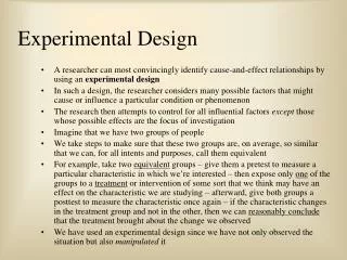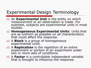
Experimental Design Terminology
Experimental Design Terminology. An Experimental Unit is the entity on which measurement or an observation is made. For example, subjects are experimental units in most studies.

Experimental Design Terminology
E N D
Presentation Transcript
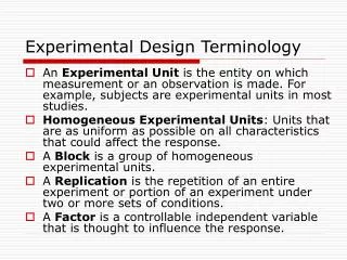
Experimental Design Terminology • An Experimental Unit is the entity on which measurement or an observation is made. For example, subjects are experimental units in most studies. • Homogeneous Experimental Units: Units that are as uniform as possible on all characteristics that could affect the response. • A Block is a group of homogeneous experimental units. • A Replication is the repetition of an entire experiment or portion of an experiment under two or more sets of conditions. • A Factor is a controllable independent variable that is thought to influence the response.
Experimental Design Terminology • Factors can be fixed or random • Fixed -- the factor can take on a discrete number of values and these are the only values of interest. • Random -- the factor can take on a wide range of values and one wants to generalize from specific values to all possible values. • Each specific value of a factor is called a level.
Experimental Design Terminology • A covariate is an independent variable not manipulated by the experimenter but still affecting the response. • Effect is the change in the average response between two factor levels. • Interaction is the joint factor effects in which the effect of each factor depends on the level of the other factors. • A Design (layout) of the experiment includes the choice of factors and factor-levels, number of replications, blocking, randomization, and the assignment of factor –level combination to experimental units.
Experimental Design Terminology • Sum of Squares (SS): Let x1, …, xn be n observations. The sum of squares of these n observations can be written as x12 + x22 +…. xn2. In notations, ∑xi2. In a corrected form this sum of squares can be written as • Degrees of freedom (df): Number of quantities of the form – Number of restrictions. For example, in the following SS, we need n quantities of the form . There is one constraint So the df for this SS is n – 1. • Mean Sum of Squares (MSS): The SS divided by it’s df.
Experimental Design Terminology • The analysis of variance (ANOVA) is a technique of decomposing the total variability of a response variable into: • Variability due to the experimental factor(s) and… • Variability due to error (i.e., factors that are not accounted for in the experimental design). • The basic purpose of ANOVA is to test the equality of several means. • A fixed effect model includes only fixed factors in the model. • A random effect model includes only random factors in the model. • A mixed effect model includes both fixed and random factors in the model.
One-way analysis of Variance • One factor of k levels or groups. E.g., 3 treatment groups in a drug study. • The main objective is to examine the equality of means of different groups. • Total variation of observations (SST) can be split in two components: variation between groups (SSG) and variation within groups (SSE). • Variation between groups is due to the difference in different groups. E.g. different treatment groups or different doses of the same treatment. • Variation within groups is the inherent variation among the observations within each group. • Completely randomized design (CRD) is an example of one-way analysis of variance.
One-way analysis of variance Consider a layout of a study with 16 subjects that intended to compare 4 treatment groups (G1-G4). Each group contains four subjects. S1 S2 S3 S4 G1 Y11 Y12 Y13 Y14 G2 Y21 Y22 Y23 Y24 G3 Y31 Y32 Y33 Y34 G4 Y41 Y42 Y43 Y44
One-way analysis of Variance • Model: • Assumptions: • Observations yij are independent. • eij are normally distributed with mean zero and constant standard deviation.
One-way analysis of Variance • Hypothesis: Ho: Means of all groups are equal. Ha: At least one of them is not equal to other. • Analysis of variance (ANOVA) Table for one way classified data
Multiple comparisons • If the F test is significant in ANOVA table, then we intend to find the pairs of groups are significantly different. Following are the commonly used procedures: • Fisher’s Least Significant Difference (LSD) • Tukey’s method • Bonferroni’s method • Scheffe’s method
One-way ANOVA - Demo • MS Excel: • Put response data (hgt) for each groups (grp) in side by side columns (see next slides) • Select Tools/Data Analysis and select Anova: Single Factor from the Analysis Tools list. Click OK. • Select Input Range (for our example a1: c21), mark on Group by columns and again mark labels in first row. • Select output range and then click on ok.
One-way ANOVA - Demo • SPSS: • Select Analyze > Compare Means > One –Way ANOVA • Select variables as Dependent List: response (hgt), and Factor: Group (grp) and then make selections as follows-click on Post Hoc and select Multiple comparisons (LSD, Tukey, Bonferroni, or Scheffe), click options and select Homogeneity of variance test, click continue and then Ok.
One-way ANOVA R output: height on treatment groups >grp<- as.factor(grp) > summary(aov(hgt~grp)) Df Sum Sq Mean Sq F value Pr(>F) grp 2 19.16 9.58 0.2803 0.7566 Residuals 57 1947.55 34.17
Analysis of variance of factorial experiment (Two or more factors) • Factorial experiment: The effects of the two or more factors including their interactions are investigated simultaneously. For example, consider two factors A and B. Then total variation of the response will be split into variation for A, variation for B, variation for their interaction AB, and variation due to error.
Analysis of variance of factorial experiment (Two or more factors) • Model with two factors (A, B) and their interactions: • Assumptions: The same as in One-way ANOVA.
Analysis of variance of factorial experiment (Two or more factors) • Null Hypotheses: • Hoa: Means of all groups of the factor A are equal. • Hob: Means of all groups of the factor B are equal. • Hoab:(αβ)ij = 0, i. e. two factors A and B are independent
Analysis of variance of factorial experiment (Two or more factors) • ANOVA for two factors A and B with their interaction AB.
Two-factor with replication - Demo • MS Excel: • Put response data for two factors like in a lay out like in the next page. • Select Tools/Data Analysis and select Anova: Two Factor with replication from the Analysis Tools list. Click OK. • Select Input Range and input the rows per sample: Number of replications (excel needs equal replications for every levels). Replication is 2 for the data in the next page. • Select output range and then click on ok.
Two-factor ANOVA MS-Excel output: height on treatment group, shades, and their interaction
Two-factor ANOVA - Demo • SPSS: • Select Analyze > General Linear Model > Univariate • Make selection of variables e.g. Dependent varaiable: response (hgt), and Fixed Factor: grp and shades. • Make other selections as follows-click on Post Hoc and select Multiple comparisons (LSD, Tukey, Bonferroni, or Scheffe), click options and select Homogeneity of variance test, click continue and then Ok.
Two-factor ANOVA SPSS output: height on treatment group, shades, and their interaction
Two-factor ANOVA R output: height on treatment group, shades, and their interaction > grp<- as.factor(grp) > shades<-as.factor(shades) > summary(aov(hgt~grp+shades+grp*shades)) Df Sum Sq Mean Sq F value Pr(>F) grp 2 19.16 9.58 0.2703 0.7642 shades 1 14.76 14.76 0.4165 0.5214 grp:shades 2 18.96 9.48 0.2674 0.7663 Residuals 54 1913.83 35.44