Download
1 / 29
290 likes | 458 Vues
Instrument Analysis Workshop I Overview of the TKR Reconstruction. Tracy Usher June 7-8, 2004 SLAC. Outline. Overview of Reconstruction General TkrRecon Strategy Overview of Tracker Reconstruction Details of Clustering Details of Track Finding Details of Track Fitting

E N D
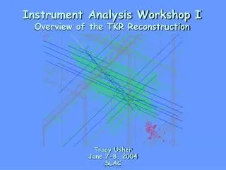
Instrument Analysis Workshop IOverview of the TKR Reconstruction Tracy Usher June 7-8, 2004SLAC
Outline • Overview of Reconstruction • General TkrRecon Strategy • Overview of Tracker Reconstruction • Details of Clustering • Details of Track Finding • Details of Track Fitting • Details of Vertexing
All algorithms run within the Gaudi Framework Reconstruction Input Sources Raw Data(Level 0) Simulation CalorimeterReconstruction TDS TrackerReconstruction Root Recon Output(Level 0.5) PersistencyService ACDReconstruction AnalysisNtuple Final Processing/Ntuple Service Reconstruction: Overview Iterative ReconTwo pass Cal & Tkr Reconis now the default mode Event Reconstruction Loop post DC-1
TkrReconGeneral Strategy • What is desired: • Basic: determine the direction of incident gamma rays converting within the tracker • In addition: help improve the determination of the incident gamma energy • Adopt four step procedure • Form “Cluster Hits” • Convert hit strips to positions • Merge adjacent hit strips to form single hit • Pattern Recognize individual tracks • Associate cluster hits into candidate tracks • Assign individual track energies • “Fit” Track to obtain track parameters • 3D position and direction • Estimated errors on above • Track fit energy estimate • “Vertex” fit tracks • Find common intersection point of fit tracks • Calculate position and resultant direction • New twist (post DC-1) • “Iterative” Recon (see next slide) • Standard HEP approach to problem
Tracker ReconSome Package Design Considerations • Goal: Easy Interchangeability • Do we have the best solutions already? • Want to be able to quickly and easily switch implementations of various algorithms • Implementation • Overall Algorithm to control Tracker Reconstruction at top level • Sub Algorithms to control each of four reconstruction steps • Gaudi Tools for specific implementation of particular task • Use TDS to store intermediate results – communicate between algorithms • Have not fully achieved goal – yet • Current structure not as transparent as would like • TDS objects need to be simplified • TkrRecon undergoing critical review amongst tracking folks now
Iterative Tracker ReconWhat and Why • What is it? • The Iterative Recon is a mechanism for allowing parts of the Tracker Reconstruction software to be called more than once per event • In particular, existing pattern recognition tracks can be refit and the vertex algorithm re-run • Why is it needed? • The Calorimeter would like the output of TkrRecon when running the energy correction algorithms. • At the same time, TkrRecon wants the best energy estimate from the Calorimeter to get the best track fits and, subsequently, the best vertices • The Iterative Recon solves this problem by providing the Calorimeter Recon with sufficient tracking information to get an improved energy estimate, which can be fed back to the track fit and vertexing algorithms • The process can be repeated as many times as the user likes (in principal)
Iterative Tracker ReconExample of Expected Improvement to Recon • Example using “WAgammas” • 1 GeV • 5° cone about normal • Into 6 m2 area containing Glast • Plot Energy of the reconstructed vertex • Red Histograms - energy of “best” vertex • Blue Histograms – include energy of second track if not part of vertex • In General • Reconstructed vertex energy improves • Some details to be understood • Shift in energy above 1 GeV probably still fallout (in this version of Gleam at least) of Tkr/Cal displacement • High energy tail? Slide circa Summer 2003
Gaudi Algorithms Implemented as Subalgorithms of TkrReconAlg TkrClusterAlgClustering of siliconstrip hits (digis) Pass 1 CalorimeterReconstruction (CalClustersAlg) Pass 1: Full Reconstruction – Clustering through Vertexing. TkrFindAlgAssociate 2D Clustersinto 3D Track Candidates Pass 1 TrackerReconstruction(TkrReconAlg) Pass 2: Track Fit and Vertexing ONLY. Assumes that improved energy reconstruction will not significantly alter the results of the track finding, so keeps the current candidate tracks. TkrTrackFitAlgFull Fit of Track CandidatesFit Method: Kalman Filter Pass 2 CalorimeterReconstruction (CalClustersAlg) Pass 2 TrackerReconstruction(TkrReconAlg) TDS TkrVertexAlgAssociate Fit Tracks toVertices and CalculateVertex Parameters Iterative Tracker ReconOverview
Strip ClusteringTkrClusterAlg • Top View looking down • Green lines represent hit strips • Blue lines are fit tracks • Yellow line is vertex vector • Red boxes are hit crystals(with some mc drawing license) • Digis give to clustering: • Hit Strip Numbers • ToT • Basic job of clustering: • Group adjacent hit strips to form cluster • Given hit strip ids, calculate cluster center position
Strip ClusteringTkrClusterAlg ToT • Close up YZ view of same event from previous page • Additional Clustering work: • Apply the Tracker “calibration” to account for hot/dead/sick strips • Merge clusters with known dead strips between them • Decide whether to add strips to clusters when known to be hot (this part tricky) • Etc. • Result of TkrClusterAlg: • List of Clusters in TDS with associated xyz coordinates and value of ToT associated with these strips One strip Cluster Measured View Two strip Cluster Non-Measured View
Pattern Recognition – Track CandidatesTkrFindAlg • The next step of TkrReconAlg is to associate clusters into candidate tracks • Note that clusters are inherently 2D • Track finding must yield 3D track candidates • Three approaches exist within the TkrRecon package • “Combo” – Combinatoric search through space points to find candidates • “Link & Tree” – Associate hits into a tree like structure • “Neural Net” • Link nearby space points forming “neurons” • link neurons by rules weighting linkages. • Also: “Monte Carlo” pattern recognition exists for testing fitting and vertexing • “Combo” method is “track by track” • Pro’s: Simple to understand (although details add complications) • Con’s: Finding “wrong” tracks early in the process throws off the rest of the track finding by mis-associating hits. Also, can be quite time consuming depending upon the depth of the search • “Link and Tree” and “Neural Net” are “global” pattern recognition techniques • Pro’s: Optimized to find tracks in entire event, less susceptible to mis-associating hits • Con’s: Both methods can be quite time consuming. In addition, “Link and Tree” (in its current implementation) operates in 2D and then requires mating to get 3D track • The “Combo” method is (still) the most advanced and best understood method • It is the default for GLAST reconstruction
First Pass Best Track Set Energies Second Pass All the others Combinatoric Pattern RecognitionOverview Calorimeter Based or Blind Search Allow up to 5 shared Clusters Hit Flagging Blind Search Global Energy Constrained Track Energy
Starting Layer: One furthest from the calorimeter • Two Strategies: • 1) Calorimeter Energy present use energy centroid (space point!) • 2) Too little Cal. Energy use only Track Hits • Work with 3D hits: • Combine clusters in adjacent x-y layers to form 3D space points Combinatoric Pattern RecognitionComboFindTrackTool “Combo” Pattern Recognition - Processing an Example Event: The Event as produce by GLEAM 100 MeV g Raw SSD Hits Slide courtesy Bill Atwood
First Guess: connect hit with Cal. Centroid Use nearestHit to find 2nd hit Sufficient Cal. Energy (42 MeV) Use Cal. centroid Combinatoric Pattern RecognitionComboFindTrackTool Slide courtesy Bill Atwood
Initial Track Guess: Connect first 2 Hits! Project and Add Hits Along the Track within Search Region The search region is set by propagating the track errors through the GLAST geometry. The default region is 9s (set very wide at this stage) Combinatoric Pattern RecognitionComboFindTrackTool Slide courtesy Bill Atwood
The Blind Search proceeds similar to the Calorimeter based Search • 1st Hit found found - tried in combinatoric order • 2nd Hit selected in combinatoric order • First two hits used to project into next layer - • 3rd Hit is searched for - • If 3rd hit found, track is built by “finding - following” as with • Calorimeter search In this way a list of tracks is formed. Crucial to success, is ordering the list! Combinatoric Pattern RecognitionComboFindTrackTool Slide courtesy Bill Atwood
Combinatoric Pattern RecognitionComboFindTrackTool Track Selection Parameter Optimization Ordering Parameter Q = Track-Quality - C1* Start-Layer - C2*First-Kink - C3*Hit-Size - C4*Leading-Hits Track_Quality: “No. Hits” - c2 : track length (track tube length) - how poorly hits fit inside it Start-Layer: Penalize tracks for starting late First-Kink: Angle between first 2 track segments / Estimated MS angle Hit-Size: Penalize tracks made up of oversized clusters (see Hit Sharing) Leading-Hits: These are unpaired X or Y hits at the start of the track. This protects against noise being preferred. Status: Current parameters set by observing studying single events. Underway – program to optimize parameters against performance metrics underway (Brian Baughman) Slide courtesy Bill Atwood
Track Finding Output • An ordered list of candidate tracks to be fit • TkrPatCand contained in a TkrPatCandCol Gaudi Object Vector • Estimated track parameters for candiate track (position, direction) • Energy assigned to the track • Track candidate “quality” estimate • Starting tower/layer information • Each TkrPatCand contains a Gaudi Object Vector of TkrPatCandHits for each hit (cluster) associated with the candidate track • Cluster associated to this hit, needed for fit stage • All stored in the TDS
Track FitTkrFitTrackAlg • The next step of TkrReconAlg is to Fit the candidate tracks • Track parameters • x, mx (slope in x direction), y, my • Track parameter error matrix (parameter errors and correlations) • Track energy (augment calorimeter estimate with fit info) • Measure of the quality of the track fit • etc. • Track Fit Method: use a Kalman Filter • Extra unnecessary details • Actually have four fitters in TkrRecon package: • Three based on Kalman Filter • KalFitTrack: also includes hit finding methods for Combo Pat Rec • KalFitter: Pure track fit using same underlying fit as above • KalmanTrackFitTool: a “generic” fitter used to cross check the above • 2D Least Squares fitter • “Classic” straight line fit
The Kalman filter process is a successive approximation scheme to estimate parameters Simple Example: 2 parameters - intercept and slope: x = x0 + Sx * z; P = (x0 , Sx) Errors on parameters x0 & Sx (covariance matrix): C = Cx-x = <(x-xm)(x-xm)> In general C = <(P - Pm)(P-Pm)T> Cx-x Cx-s Cs-x Cs-s Propagation: x(k+1) = x(k)+Sx(k)*(z(k+1)-z(k)) Pm(k+1) = F(dz) * P(k) where F(dz) = Pm(k+1) P(k) 1 z(k+1)-z(k) 0 1 k+1 Cm(k+1) = F(dz) *C(k) * F(dz)T + Q(k) Noise: Q(k) (Multiple Scattering) k Track Fitting:The Kalman Filter Slide courtesy Bill Atwood
Form the weighted average of the k+1 measurement and the propagated track model: Weights given by inverse of Error Matrix: C-1 Pm(k+1) Hit: X(k+1) with errors V(k+1) k+1 Noise (Multiple Scattering) k Cm-1(k+1)*Pm(k+1)+ V-1(k+1)*X(k+1) P(k+1) = and C(k+1) = (Cm-1(k+1) + V-1(k+1))-1 Cm-1(k+1) + V-1(k+1) Now its repeated for the k+2 planes and so - on. This is called FILTERING - each successive step incorporates the knowledge of previous steps as allowed for by the NOISE and the aggregate sum of the previous hits. Track Fitting:The Kalman Filter Slide courtesy Bill Atwood
Track Fitting:The Kalman Filter We start the FILTER process at the conversion point BUT… We want the best estimate of the track parameters at the conversion point. Must propagate the influence of all the subsequent Hits backwards to the beginning of the track - Essentially running the FILTER in reverse. This is call the SMOOTHER & the linear algebra is similar. Residuals & c2: Residuals: r(k) = X(k) - Pm(k) Covariance of r(k): Cr(k) = V(k) - C(k) Then: c2 = r(k)TCr(k)-1r(k) for the kth step Slide courtesy Bill Atwood
All declared explicitly in the TDSGenerally considered overly complicated – undergoing review now (again) Event::TkrKalFitTrack • Repeated for each phase of the Kalman Fit: • Measured • Prediction • Filtering • Smoothing Event::TkrFitTrackBase Event::TkrFitPlaneCol(ObjectVector<TkrFitPlane>) Event::TkrFitPlane Event::TkrFitPar ContainedObject Event::TkrFitHit Event::TkrFitMatrix Track Fit Output
“Vertexing”TkrVertexAlg • Assume Gamma conversion results in 1-2 primary tracks • 1 track in pair conversion could be lost • Too low energy (track must cross three planes) • Tracks from pair conversion don’t separate for several layers • Track separation due to multiple scattering • etc. • Secondary tracks associated with primary tracks, not part of gamma conversion process • Task of the vertexing algorithm • Attempt to associate “best” track (from track finding) with one of the other found tracks • Finds “the” gamma vertex • Unassociated (“Isolated”) tracks returned as single prong vertices • Determine the reconstructed position of the conversion • Determine the reconstructed direction of the conversion • Currently two methods available: • “Combo” Vertex Tool (the default for Gleam) • Uses track Distance of Closest Approach (DOCA) to associate tracks • Kalman Filter Vertex Tool (Not used, still under development) • Uses a Kalman Filter to associate tracks
“Combo” Vertex Reconstruction • Vertex determined at two track Distance of Closest Approach (DOCA) • First track is “best” track from track finding/fitting • Loop through “other” tracks looking for best match: • Smallest DOCA • Weighting factor • Separation between the starting points of the two tracks • Track energy • Track quality • Calculate Vertex quantities • Vertex Position • Midpoint of DOCA vector • Vertex Direction • Weighted vector sum of individual track directions • Not a true HEP Vertex Fit
ComboVtxTool Resulting Vertex “left” track “right” track
DOCA VertexingIllustration of Parallel Track Problem • Parallel (or close) tracks can be problematic • Direction probably very good • Vertex position can easily be significantly off • (from previous example!) Reconstructed Vertex position Two very nearly parallel tracks (sharing the same first cluster)
Vertexing Output • An ordered list of vertices • TkrVertex objects contained in a Gaudi Object Vector • Vertex Track Parameters • (x, mx, y, my) • Vertex Track Parameter covariance matrix • Vertex Energy • Vertex Quality • First tower/layer information • Gaudi Reference vector to the tracks in the vertex • First Vertex in the list is the “best” vertex • Mostly the rest are associated with “isolated” tracks
Overview of TkrReconThe End • Very General Overview of TkrRecon • Hopefully provides a roadmap for people to start digging in • Current structure of Algorithms, Tools and interfaces is somewhat complicated • Hope to simplify this over the summer as we prepare for DC-2 • No Discussion of Output Ntuple • Personal bias: Can’t do detailed studies of Tracker performance from ntuple alone • Must dig into the TDS/PDS output • No Discussion of Monte Carlo relational tables • A separate talk by itself • Don’t be afraid to ask questions! • More eyes looking at things is good • Valuable feedback on how to improve things