Download
1 / 59
590 likes | 781 Vues
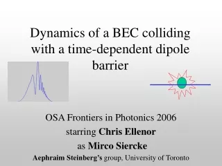
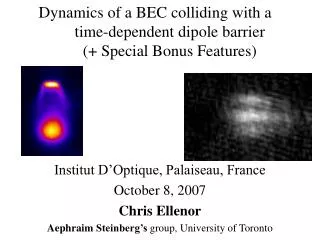
Institut D’Optique, Palaiseau, France October 8, 2007 Chris Ellenor Aephraim Steinberg’s group, University of Toronto. Dynamics of a BEC colliding with a time-dependent dipole barrier (+ Special Bonus Features). DRAMATIS PERSONÆ Toronto quantum optics & cold atoms group:

E N D
Institut D’Optique, Palaiseau, France October 8, 2007 Chris Ellenor AephraimSteinberg’s group, University of Toronto Dynamics of a BEC colliding with a time-dependent dipole barrier(+ Special Bonus Features)
DRAMATIS PERSONÆ Toronto quantum optics & cold atoms group: Postdocs: An-Ning Zhang( IQIS) Morgan Mitchell ( ICFO) (HIRING!) Matt Partlow(Energetiq)Marcelo Martinelli ( USP) Optics: Rob Adamson Kevin Resch(Wien UQIQC) Lynden(Krister) Shalm Jeff Lundeen (Oxford) Xingxing Xing Atoms: Jalani Fox (Imperial) Stefan Myrskog (BEC ECE) (SEARCHING!)Mirco Siercke ( ...?) Ana Jofre(NIST UNC) Samansa ManeshiChris Ellenor Rockson ChangChao ZhuangXiaoxian Liu UG’s:Ardavan Darabi, Nan Yang, Max Touzel, Michael Sitwell, Eugen Friesen Some helpful theorists: Pete Turner, Michael Spanner, H. Wiseman, J. Bergou, M. Mohseni, J. Sipe, Daniel James, Paul Brumer, ...
Talk Outline • BEC Experiment: Dynamics of a BEC colliding with a time-dependent dipole barrier • Motivation: Tunneling • The “Muga” Effect • Applications to state measurement / tomography • Some ground (by “ground” I mean “experiment”) breaking data • Lattice Experiment: Decoherence and Control of Vibrational States of Atoms in an Optical Lattice
Motivation • Our long term goal is to study transit times for atoms tunneling through a potential barrier • To begin, we will study predictions of non-classical behaviour in collisions with this barrier • This effect suggests an interferometric method for measuring the condensate wavefunction / Wigner function
Collisional Transitory Enhancement of the High Momentum Components of a Quantum Wave Packet • S. Brouard and J. G. Muga, Phys. Rev. Lett. 81, 2621–2625 (1998)
Collisional Transitory Enhancement of the High Momentum Components of a Quantum Wave Packet • S. Brouard and J. G. Muga, Phys. Rev. Lett. 81, 2621–2625 (1998)
Collisional Transitory Enhancement of the High Momentum Components of a Quantum Wave Packet • S. Brouard and J. G. Muga, Phys. Rev. Lett. 81, 2621–2625 (1998) accumulated probability for momentum > p • Consider an ensemble of particles with some distribution in phase space approaching a repulsive potential • Classically, we can construct the inequality • Quantum mechanically, this can be violated, and higher momentum components produced, i.e. G > 0 More localized = higher momentum components incoming outgoing
In our experiment we’ll use a small, weak barrier that barely causes any reflection of the BEC to look for these transient effects. (Brouard S., Muga J.G., Annalen der Physik 7 (7-8): 679-686 1998) We will switch the barrier off, let the BEC expand and get the momentum distribution from the time of flight Collisional transitory enhancement of the high momentum components Momentum distributions:
This effect can be easily understood by realizing that the barrier writes a Pi phaseshift onto the wavefunction • The effect is a single-particle effect, so mean field energy present would make it impossible to use time of flight measurements to extract momentum distributions, and soliton formation would further complicate matters
Performing the experiment with an expanded BEC: 0 ms drop before collision Variable barrier position = variable drop time before collision TOF measurement of momentum distribution at time of collision
Performing the experiment with an expanded BEC: 1 ms drop before collision Variable barrier position = variable drop time before collision TOF measurement of momentum distribution at time of collision
Performing the experiment with an expanded BEC: 5 ms drop before collision Variable barrier position = variable drop time before collision TOF measurement of momentum distribution at time of collision
Performing the experiment with an expanded BEC: 12 ms drop before collision Variable barrier position = variable drop time before collision TOF measurement of momentum distribution at time of collision
One can think of the expanded BEC as a series of transform-limited wavepackets each with a different phase and velocity • The fast wavepackets picked up a total phase of pi, the slow ones no phase, and only the central one exhibits transient enhancement of momentum
The fringes then tell us the phase difference between the central momentum component and the rest of the cloud, allowing reconstruction of the wavefunction
Tomography? • For a pure state, one shot should be enough • For a mixed state, taking measurements at different times (different collision times) should be enough to assemble a Wigner function (but we’re not sure how) • Maybe able to achieve excellent position resolution of initial state by measuring phase well • Also could watch evolution of “purity,” e.g. in the Mott insulator transition’ • Initial position of cloud has been offset by 1mm • Could distinguish coherent vs. incoherent addition
Frequency-Resolved Optical Gating (FROG) “Polarization-Gate” Geometry Spectro- meter Trebino, et al., Rev. Sci. Instr., 68, 3277 (1997). Kane and Trebino, Opt. Lett., 18, 823 (1993).
Some preliminary data • 5.6ms expansion before collision, 15ms expansion after
Comparing to numerical models • (Change the phase shift given by the barrier) (Ok – Maybe a bit of wishful thinking!)
AOM FPGA The Dipole Barrier – Making a Sheet of Light Absorption probe 200 GHz detuned laser diode
AOM FPGA The Dipole Barrier – Making a Sheet of Light Absorption probe AOM scans beam
AOM FPGA The Dipole Barrier – Making a Sheet of Light Absorption probe BEC of about 10587Rb atoms Spot is 8um thick by 200um wide With scan - sheet is ~ 0.5mm wide Height is ~ 150nK Intensity flat to < 1%
Part 1 Summary • During the collision of a wavepacket with a barrier transient effects can be observed that are not visible in the asymptotic scattering limits. • We may realize an interferometric effect similar to FROG where we infer phase information, and perhaps the Wigner function of our BEC using these transient effects • Preliminary results have been achieved, possibly demonstrating a new technique for extraction of phase information from a condensate • Possible applications to BEC tomography, and study of entanglement evolution
Talk Outline • BEC Experiment: Dynamics of a BEC colliding with a time-dependent dipole barrier • Motivation: Tunneling • The “Muga” Effect • Applications to state measurement / tomography • Some ground (by “ground” I mean “experiment”) breaking data • Lattice Experiment: Decoherence and Control of Vibrational States of Atoms in an Optical Lattice • Preparing and tomographing quantum states in an optical lattice • Atom (pulse) echoes • Designer excitation pulses • Probing decoherence with 2-D pump-probe spectroscopy • Coherent control of vibrational excitations
AOM2 PBS TUI Amplifier Grating Stabilized Laser AOM1 PBS PBS Spatial filter Function Generator Controlling phase of AOMs allows control of lattice position Vertical1DOptical Lattice Experimental Setup Cold 85Rb atoms T~10μK Lattice spacing : a ~ 0.93μm Effective lattice recoil energy = ER~ 32nK Uo =(18-20)ER = (580-640)nK
1 Quantum CAT scans
Tomography & control in Lattices [Myrkog et al., PRA 72, 013615 (05) Kanem et al., J. Opt. B7, S705 (05)] Rb atom trapped in one of the quantum levels of a periodic potential formed by standing light field (30GHz detuning, c. 20 ER in depth) Goals: How to fully characterize time-evolution due to lattice? How to correct for “errors” (preserve coherence,...)?
Basic Ingredients for Tomography • State Preparation • State Measurement • Unitary operations, i.e. Measure in different bases
Initial Lattice After adiabatic decrease Well Depth 0 t1 t1+40ms t(ms) Preparing a ground state 2 bound states 1 bound state 7 ms 0 to to+30ms Measuring State Populations Ground State 1st Excited State
Atomic state measurement(for a 2-state lattice, with c0|0> + c1|1>) initial state displaced delayed & displaced left in ground band tunnels out during adiabatic lowering (escaped during preparation) |c0 + i c1 |2 |c0|2 |c0 + c1 |2 |c1|2
Extracting a superoperator:prepare a complete set of input states and measure each output Likely sources of decoherence/dephasing: Real photon scattering (100 ms; shouldn't be relevant in 150 s period) Inter-well tunneling (10s of ms; would love to see it) Beam inhomogeneities (expected several ms, but are probably wrong) Parametric heating (unlikely; no change in diagonals) Other
Quantum state reconstruction D x Wait… Shift… 1 1 p p Q(0,0) = P g n W(0,0) = (-1) P S Measure ground state population n (former for HO only; latter requires only symmetry) Cf. Poyatos,Walser,Cirac,Zoller,Blatt, PRA 53, 1966 ('96) & Liebfried,Meekhof,King,Monroe,Itano,Wineland, PRL77, 4281 ('96)
Data:"W-like" [Pg-Pe](x,p) for a mostly-excited incoherent mixture
2 Atom echoes
Oscillations in lattice wells (Direct probe of centre-of-mass oscillations in 1mm wells; can be thought of as Ramsey fringes or Raman pump-probe exp’t.)
Towards bang-bang error-correction:pulse echo indicates T2 ≈ 1 ms... 0 500 ms 1000 ms 1500 ms 2000 ms coherence introduced by echo pulses themselves (since they are not perfect p-pulses) Free-induction-decay signal for comparison echo after “bang” at 800 ms echo after “bang” at 1200 ms echo after “bang” at 1600 ms (bang!)
Echo from compound pulse Pulse 900 us after state preparation, and track oscillations single-shift echo (≈10% of initial oscillations) double-shift echo (≈20-30% of initial oscillations) Ongoing: More parameters; find best pulse. E.g., combine amplitude & phase mod. Also: optimize # of pulses. time ( microseconds)
Cf. Hannover experiment Far smaller echo, but far better signal-to-noise ("classical" measurement of <X>) Much shorter coherence time, but roughly same number of periods – dominated by anharmonicity, irrelevant in our case. Buchkremer, Dumke, Levsen, Birkl, and Ertmer, PRL 85, 3121 (2000).
Why does our echo decay? 3D lattice (preliminary results) Except for one minor disturbing feature: These data were first taken without the 3D lattice, and we don’t have the slightest idea what that plateau means. (Work with Daniel James to relate it to autocorrelation properties of our noise, but so far no understanding of why it’s as it is.) Present best guess = finite bath memory time: So far, our atoms are free to move in the directions transverse to our lattice. In 1 ms, they move far enough to see the oscillation frequency change by about 10%... which is about 1 kHz, and hence enough to dephase them.
3 Our thinking shows one-dimensionality
wexc wdet wexc wexc wdet wdet