Estimating and Testing Mediation

1. Estimating and Testing Mediation • David A. Kenny • University of Connecticut • http://davidakenny.net/cm/MediationN.ppt

2. Overview • Introduction (click to go there) • The Four-Step Approach (click) • The Modern Approach (click) • Test the Indirect Effect (click) • Power (click) • Assumptions(click) • DataToText (click)

3. Introduction

4. Interest in Mediation Mentions of “mediation” or “mediator” in psychology abstracts: 1980: 36 1990: 122 2000: 339 2010: 1,198 4

5. Why the Interest in Mediation? • Understand the mechanism • theoretical concerns • cost and efficiency concerns • Find more proximal endpoints • Understand why the intervention did not work • finding the missing link • compensatory processes

6. The Beginning Model:Basic Research c Y X

7. The Mediational Model M b a c' Y X

8. The Beginning Model:Applied Research M b Y

9. The Four Paths • X  Y: path c • X  M: path a • M  Y (controlling for X): path b • X  Y (controlling for M): path c′ (standardized or unstandardized)

10. The Four-Step Approach

11. In the 1980s Different Pairs of Researchers Proposed a Series of Steps to Test Mediation • Judd & Kenny (1981) • James & Brett (1984) • Baron & Kenny (1986)

12. The Four Steps • Step 1: X Y (test path c) • Step 2: X M (test path a) • Step 3: M(and X) Y (test path b) • Step 4: X (and M) Y (test path c′) Note that Steps 3 and 4 use the same regression equation.

13. Total and Partial Mediation • Total Mediation • Meet steps 1, 2, and 3 and find that c′ equal zero. • Partial Mediation • Meet steps 1, 2, and 3 and find that c′ is smaller in absolute value than c.

14. Example Dataset • Morse et al. • J. of Community Psychology, 1994 • treatment  housing contacts  days of stable housing • persons randomly assigned to treatment groups. • 109 people (davidakenny.net/papers/twmr/example.txt)

15. Variables in the Example • Treatment • 1 = treated (intensive case management) • 0 = treatment as usual • Housing Contacts: total number of contacts per during the 9 months after the intervention began • Stable Housing • days per month with adequate housing (0 to 30) • Averaged over 7 months from month 10 to month 16, after the intervention began

16. Morse et al. Example • Step 1: X  Y • c = 6.558, p = .009 • Step 2: X  M • a = 5.502, p = .013 • Step 3: M (and X)  Y • b = 0.466, p < .001 • Step 4: X (and M)  Y • c′ = 3.992, p = .090

17. When Can We Conclude Complete Mediation? When c′ is not statistically different from zero, but c is? NOT REALLY Ideally when a and b are substantial and c′ is small, not just non-significant.

18. Standardized vs. Unstandardized For most everything in this presentation, the variables can be standardized making the coefficients Betas. The key thing is to be consistent: If M is standardized in Step 2, it is also standardized in Step 3.

19. Presenting Mediation 19

20. The Modern Approach

21. Dissatisfaction with the Steps Approach Low power in the test of Step 1 No single measure and test of mediation Work by MacKinnon, Hayes, Preacher and others has led to the “Modern Approach.”

22. Decomposition of Effects Total Effect = Direct Effect + Indirect Effect c = c′ + ab This equality exactly holds for multiple regression, but not necessarily for other estimation methods. The Indirect Effect or ab provides one number that summarizes the amount of mediation. Example: 6.558 = 5.502x 0.466 And 100(2.56/6.56) = 39% of the total effect is explained (ab/c or equivalently 1 - c′/c).

23. Two Sides of the Same Coin Note that ab = c - c′ That is, the indirect effect exactly equals the amount of the reduction in the total effect (c) after the mediator is introduced. Some papers (e.g., Baron & Kenny) emphasize one side and others emphasize the other. Current work in mediation is now focused on the “ab” side.

24. Estimating the Total Effect (c) The total effect or c can be inferred from direct and indirect effect as c′ + ab. We need not perform the Step 1 regression to estimate c. This can be useful in situations when c does not exactly equally c′ + ab.

25. What to Present Decomposition of Effects Total Effect Indirect Effect(s) Direct Effects Less of an emphasis on complete versus partial mediation.

26. Test of the Indirect Effect

27. Work on Determining How to Test ab = 0 The key piece of information in the modern approach is the indirect effect. Many researchers developed approaches to this problem. 27

28. Strategies to Test ab = 0 • Test a and b separately • Sobel test • Bootstrapping • Monte Carlo Method

29. Test a and b Separately • Easy to do • Works fairly well • Does not provide a method for a confidence interval for ab. • Seem too much like the old-fashioned Four-Step Approach.

30. Sobel Test of Mediation Compute the square root of a2sb2 + b2sa2 which is denoted as sab Note that sa and sb are the standard errors of a and b, respectively; ta = a/sa and tb = b/sb. Divide ab by sab and treat that value as a Z. So if ab/sab greater than 1.96 in absolute value, reject the null hypothesis that the indirect effect is zero.

31. Example a = 5.502 and b = 0.466 sa = 2.182 and sb = 0.100 ab = 2.56; sab = 1.157 Sobel test Z is 2.218, p = .027 We conclude that the indirect effect is statistically different from zero. Website: http://www.people.ku.edu/~preacher/sobel/sobel.htm

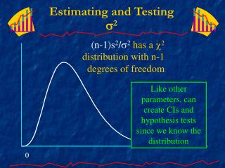
32. Large values of “ab” are more variable than small values (i.e., 0). 0 ab The distribution of ab is highly skewed which lowers the power of the test.

33. Bootstrapping • “Nonparametric” way of computing a sampling distribution. • Re-sampling (with replacement) • Many trials (computationally intensive) • Current thinking is NOT to correct for bias (i.e., the mean of the bootstrap estimate differs slightly from the estimate). • Compute a confidence interval which is asymmetric. • Slight changes because empirically derived.

34. Results of Bootstrapping 95% Percentile Confidence Interval: Lower Upper .5325 5.0341 Note that the CI is asymmetric for an estimate of 2.598. Also values differ to sampling error. (Done using the Hayes & Preacher macro from http://www.afhayes.com/spss-sas-and-mplus-macros-and-code.html.)

35. Monte Carlo Method • Save a, b, sa (the standard error of a) and sb from the mediation analysis. • For some methods you have the covariance of ab or sab to save. • Use them and the assumption of normality to generate estimates of a and b and so ab. • Use this distribution of ab’s to get a confidence interval or a p value. • Less computationally intensive than bootstrapping and many trials are feasible.

36. Results of the Monte Carlo Method 95% Monte Carlo Confidence Interval (20,000 trials): Lower Upper 0.551 5.158 Done using the Selig & Preacher web program at http://www.quantpsy.org/medmc/medmc.htm; if correlated use Tofighi’s Rmediation at http://www.amp.gatech.edu/RMediation

37. Power

38. Power and the Test of c If c′ is zero, then c equals ab. If both a and b have a moderate effect size, then c has a “smaller than small” effect size (assuming c′ is zero). Thus, it is very possible to have tests of significance for a and b be statistically significant, but c is not. Note that for the example if a and b have moderate effect sizes (r = .3) and c′ = 0, the power of the test of c is only .15.

39. Relative Power of c and ab Several authors, as early as Cox (1960), have noted that the indirect effect has much more power than the test of c even when the two equal the same value as when c′ is zero, then c equals ab. equals zero. As Kenny and Judd (2014) showed, sometimes the indirect the test of c need 75 times the number of cases to have the same power as the test of ab!

40. Power and the Test of c′ When b = 0, c = c′ and in this case c might be statistically significant, yet c′ might not be significant even though. Why? There is multicollinearity between X and M due to path a. Note that as M becomes a more successful mediator and path a gets larger, multicollinearity becomes more of a issue in the testing of c′ (and b).

41. Power and the Test of b Test of path a has more power than the test of path b (b = .3, standardized): aN .1 86 .3 93 .5 112 (a is standardized; sample size needed for 80% power to reject the null hypothesis that b = 0) Conclusion: Power of the test of b declines as a increases.

42. Tool MedPowR R based program to help in power analyses. Can either give the power for a given value of N and a, b, and c’ or give the N needed to achieve a desired level of power. Program can be downloaded at http://davidakenny.net/progs/PowMed.R

44. Power calculations have begun... Effect Size Power N c .390 .986 100 a .300 .868 100 b .300 .890 100 c' .300 .890 100 ab .090 .773 100 Alpha for all power calculations set to .050. Power calculations complete.

45. Assumptions

46. Taking Assumptions Seriously Older Mediation Analysis ignored the strong assumptions required for the analysis. Current work, especially that within the Causal Inference tradition, focuses much more on them. Researchers need to conduct “Sensitivity Analyses” or “What If?”analyses. 46

47. Assumptions: Multiple Regression Linearity Is a problem in the example; housing contacts has a quadratic effect on stable housing (p = .034). Normal Distribution of Errors Interval level of measurement of M and Y Equal Error Variance Independence No clustering X and M Do Not Interact to Cause Y 47

48. No XM Interaction: Linear Mediation • Called “Moderation” in Baron & Kenny • Add XM (and possibly other interaction terms, e.g., X2M) when explaining Y. • Many contemporary analysts now see XM interaction as part of mediation. • Not significant for the example (p = .476)

49. Causal Assumptions Perfect Reliability for M and X M and Y not cause X No Omitted Variables all common causes of M and Y, X and M, and X and Y measured and controlled No Reverse Causal Effects Y may not cause M (Guaranteed if X is manipulated.) 49

50. Basic Mediational Causal Model Note that U1 and U2 are theoretical variables and not “errors” from a regression equation.