Download
1 / 32
320 likes | 341 Vues
This analysis discusses the O-GEHL branch predictor, a high-performance and power-efficient solution for improving branch prediction accuracy in long pipelines with multiple instructions per cycle. The predictor utilizes a combination of global and local history, adaptive history length fitting, and an adder tree for selecting between predictions. The analysis explores the impact of history length choices, the number of components, and counter width on the accuracy of the predictor. The O-GEHL predictor proves to be a robust and efficient solution for branch prediction.

E N D
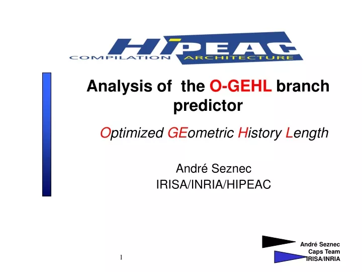
Analysis of the O-GEHL branch predictor Optimized GEometric History Length André Seznec IRISA/INRIA/HIPEAC
Branch prediction is still an issue • Long pipelines • Several instructions per cycle • Any gain in branch prediction accuracy results in: • Performance gain • Power consumption gain
Conditional branch predictors 25 years of background work • Two main sources of information: • Local history • the past behavior of this particular branch • Global history • the (recent) past behavior of all branches
Speculative history must be managed !? • Global history: • Append a bit on asinglehistory register • Use of a circular buffer and just a pointer to speculatively manage the history • Local history: • table of histories (unspeculatively updated) • must maintain a speculative history per inflight branch: • Associative search, etc ?!?
From my experience with EV8 team Designers hate maintaining speculative local history
“Classical” stuff with the OGEHL predictor • Global history based: • Yeh and Patt 91, Pan and So 91 • Multiple tables using different history lengths • McFarling 93, Evers et al. 96, EV8 predictor
Selecting between multiple predictions • Classic solution: • Use of a meta predictor “wasting” storage !?! chosing among 5 or 10 predictions ?? • Neural inspired predictors: • Use an adder tree instead of a meta-predictor Vintan and Iridon 99, Jiménez and Lin 01 Let’s use the adder tree
TO T1 T2 ∑ T3 L(1) L(2) T4 L(3) L(4) Multiple history length predictor Final computation through a sum L(0) Prediction=Sign
GEometric History Length predictor The set of history lengths forms a geometric series {0, 2, 4, 8, 16, 32, 64, 128} What is important:L(i)-L(i-1) is drastically increasing Spends most of the storage for short history !!
Dynamic update threshold fitting Reasonable fixed threshold= Number of tables On an O-GEHL predictor, best threshold depends on • the application • the predictor size • the counter width By chance, on most applications, for the best fixed threshold, updates on mispredictions ≈ updates on correct predictions Monitor the difference and adapt the update threshold
(½ applications: L(7) < 50) ≠ (½ applications: L(7) > 150) Let us adapt some history lengths to the behavior of each application 8 tables: T2: L(2) and L(8) T4: L(4) and L(9) T6: L(6) and L(10) Adaptative history length fitting (inspired by Juan et al 98)
Adaptative history length fitting (2) Intuition: • if high degree of conflicts on T7, stick with short history Implementation: • monitoring of aliasing on updates on T7 through a tag bit and a counter Simple is sufficient: • Flipping from short to long histories and vice-versa
TO T1 T2 L(0) ∑ T3 L(1) or L(5) L(2) T4 L(3) or L(6) L(4) Tag bits
Hashing 200+ bits for indexing !! • Need to compute 11 bits indexes : • Full hashing is unrealistic • Just regularly pick at most 33 bits in: address+branch history +path history • A single 3-entry exclusive-OR stage
Evaluation framework 1st Championship Branch Prediction traces: 20 traces including system activity Floating point apps : loop dominated Integer apps: usual SPECINT Multimedia apps Server workload apps: very large footprint
Reference configurationpresented for Championship Branch Prediction • 8 tables: • 2 Kentries except T1, 1Kentries • 5 bit counters for T0 and T1, 4 bit counters otherwise • 1 Kbits of one bit tags associated with T7 10K + 5K + 6x8K + 1K = 64K • L(1) =3 and L(10)= 200 • {0,3,5,8,12,19,31,49,75,125,200}
A case for the OGEHL predictor • 2nd at CBP: 2.82 misp/KI • Best practice award: • The predictor the closest to a possible hardware implementation • Does not use exotic features: • Various prime numbers, etc • Strange initial state • Chaining simulations: 2.84 misp/KI • Very fast warming
A case for the OGEHL predictor (2) • High accuracy • 32Kbits (3,150): 3.41 misp/KI better than any implementable 128 Kbits predictor before CBP • 128 Kbits 2bcgkew (6,6,24,48): 3.55 misp/KI • 176 Kbits PBNP (43) : 3.67 misp/KI • 1Mbits (5,300): 2.27 misp/KI • 1Mbit 2bcgskew (9,9,36,72): 3.19 misp/KI • 1888 Kbits PBNP (58): 3.23 misp/KI
A case for the OGEHL predictor (3) • Robustness to variations of history lengths choices: • L(1) in [2,6], L(10) in [125,300] • misp. rate < 2.96 misp/KI • Geometric series: not a bad formula !! • best geometric L(1)=3, L(10)=223, 2.80 misp/KI • best overall {0, 2, 4, 9, 12, 18, 31, 54, 114, 145, 266} 2.78 misp/KI
Impact of the number of components • 4 components — 8 components • 64 Kbits: 3.02 -- 2.84 misp/KI • 256Kbits: 2.59 -- 2.44 misp/KI • 1Mbit: 2.40 -- 2.27 misp/KI • 6 components — 12 components • 48 Kbits: 3.02 – 3.03 misp/KI • 768Kbits: 2.35 – 2.25 misp/KI 4 to 12 components bring high accuracy
Impact of counter width • Robustness to counter width variations: • 3-bit counter, 49 Kbits: 3.09 misp/KI Dynamic update threshold fitting helps a lot • 5-bit counter 79 Kbits: 2.79 misp/KI 4-bit is the best tradeoff
Prediction computation time • 3 successive steps: • Index computation: a 3-entry XOR gate • Table read • Adder tree • May not fit on a single cycle: • But can be ahead pipelined !
Ahead pipelining a global history branch predictor (principle) • Initiate branch prediction X+1 cycles in advance to provide the prediction in time • Use information available: • X-block ahead instruction address • X-block ahead history • To ensure accuracy: • Use intermediate path information
A B C D bcd Practice Ahead OGEHL: 8 // prediction computations Ha A
Ahead Pipelined 64 Kbits OGEHL • 3-block: 2.94 misp/KI • 4-block: 2.99 misp/KI • 5-block: 3.04 misp/KI Not such a huge accuracy loss
A final case for the O-GEHL predictor • delivers state-of-the-art accuracy • uses only global information: • Very long history: 200+ bits !! • can be ahead pipelined • many effective design points • Nb of tables, counter width, history lengths • prediction computation logic complexity is low (compared with concurrent predictors)
Still open questions • Does it exist better prediction combination functions ? • Indirect jump targets ?
Improved the global history • Address + conditional branch history: • path confusion on short histories • Address + path: • Direct hashing leads to path confusion • Represent all branches in branch history • Use also path history ( 1 bit per branch, limited to 16 bits)
Piecewise linear -- OGEHL (1) accuracy • My own best implementation of piecewise linear: • Shares counters for the same history rank • but uses only power of two numbers of entries in tables • 64 Kbits: H=31, 256 counters per rank, x 32 sums • 3.72 misp/KI ------------ 2.84 misp/KI • 1 MBit : H=63, 2048 counters per rank, x 32 sums • 2.64 misp/KI ------------ 2.27 misp/KI • 48 Mbit: H=95, 64K counters per rank, x 32 sums • 2.30 misp/KI
Piecewise linear -- OGEHL (2) hardware complexity • Computation logic complexity: • OGEHL: only a few adders • PL: hundreds of adders • Number of storage tables • OGEHL: 4 to 12 • PL: H tables ( update time) • Prediction computation time: • + a 3-entry XOR gate on OGEHL • Information to checkpoint: • Kilobits for PL