Ant Colony Optimisation
Ant Colony Optimisation. Dr Jonathan Thompson, School of Mathematics, Cardiff University. Outline. Introduction to ant algorithms Overview of implementation for TSP (Dorigo et al.) Application to Dynamic Vehicle Routing (Wallace and Thompson) Application to Room Fitting (Thompson)


Ant Colony Optimisation
E N D
Presentation Transcript
Ant Colony Optimisation Dr Jonathan Thompson, School of Mathematics, Cardiff University SWORDS 2004
Outline • Introduction to ant algorithms • Overview of implementation for TSP (Dorigo et al.) • Application to Dynamic Vehicle Routing (Wallace and Thompson) • Application to Room Fitting (Thompson) • Application to Examination Timetabling / Graph Colouring (Dowsland and Thompson) • Conclusions SWORDS 2004
Classification of Meta-heuristics Osman divided meta-heuristics into: • Local search • Population • Construction SWORDS 2004
Solution Space Feasible regions SWORDS 2004
Local Search Solution Space SWORDS 2004
Local Search Solution Space SWORDS 2004
Local Search Solution Space SWORDS 2004
Population Based Solution Space SWORDS 2004
Population Based Solution Space SWORDS 2004
Construction Solution Space SWORDS 2004
Construction Solution Space SWORDS 2004
Construction Solution Space SWORDS 2004
Ant Algorithms SWORDS 2004
The Ant System in Nature SWORDS 2004
Ant Algorithms • Proposed by Dorigo et al. • Probabilistic greedy construction heuristic • Probabilities are adjusted according to information on solution quality gained from previous solutions • Initially use limited to routing problems but now being applied to a broad range of problems. SWORDS 2004
Ant Systems for the TSP • No. ants = No. cities • Each ant i produces a (probabilistic) solution, cost ci • Trail between each pair of cities in route i = trail + Q/ci • Trail is subject to evaporation i.e. trail = trail * σ, σ < 1 • Each ant chooses next city with a probability proportional to the distance and the trail. SWORDS 2004
Ants for TSP • Probability of next city from i being k is P(ik) = [ik] [ik] [jk] [jk] where μik = Q / distance from i to k, ik = trail between i and k. • Continues through generations until reaches stagnation • Has outperformed other meta-heuristics SWORDS 2004
The Static VRP • A set of geographically dispersed customers need to be serviced. • All routes start and end at the depot. • A cost cij, is associated with travelling from customer i to customer j. • Customer i has demand Di, vehicles have capacity Q • Construct a set of routes such that cost is minimised and each customer is visited once and capacity constraints are satisfied. SWORDS 2004
Example VRP SWORDS 2004
Adding Dynamism (DVRP) • Static VRP • Customers are known a priori and do not change after the routes have been constructed. • Dynamic VRP • Customers can change after the initial routes have been constructed. SWORDS 2004
Graphically Explained New Customer Arrives What happens now ? SWORDS 2004
Two Solution Approaches • Insertion Heuristics • Insert the new customers in the current routes. • Improvement heuristics when system is idle. • Re-Optimization i.e. solve static VRPs • Re-planning from scratch when new information is received / after each time period. SWORDS 2004
Graphically Explained – Re-Opt New Customer Arrives Current route is discarded. If capacity is not exceeded then a new route is created. If exceeded then new routes are constructed SWORDS 2004
ACS-DVRP Pseudo-code • Overnight, an initial solution is created and commit drivers to customers for first time period + small commitment time. • Each time period is then considered in turn. • Customers = existing customers who have not been committed to + new customers who arrived during the previous time slot. • Solve problem during current time period and commit drivers to customers if start time is within the subsequent time period • Continue until all customers are committed to. SWORDS 2004
Roulette Wheel Choice A schedule is being created, truck is at customer i. A roulette wheel type selection is made to decide where to go next. Size of the slot depends on attractiveness of the move. SWORDS 2004
Ants for the DVRP (ACS-DVRP) Better solutions obtained by: • Diversification: local trail update ij = (1 – ρ) ij + ρ 0 • Select best choice with probability q, probabilistically with probability (1 – q). • Elitism – only use best ant solution to update trail globally • Maintain trails from one problem to another ij = (1 – γ) ij + γ 0 • Apply descent to each ant solution • Full parameter optimisation SWORDS 2004
Preliminary Results 3 Data Sets Min, Ave, Max SWORDS 2004
Problems with the ACS-DVRP • Sequential route construction: • Each route is completed before the next is created. • Customers may be scheduled in an early truck, though may have been better placed in a later one. • High variance within results: • Difficult to interpret results. • Minimized through use of trials. SWORDS 2004
Extended Roulette Wheel Consider more than 1 truck at a time. Consider 3 trucks, 1 at customer i, 1 at customer j and 1 at the depot Arcs that would have been ignored previously are now considered. SWORDS 2004
Extended Roulette Wheel Results Why ? An increase in the number of trucks used. SWORDS 2004
Truck Reduction Techniques • Capacity Utilization. • Encourages the use of existing trucks over the selection of a new truck. • Let kij=(Qi+qj)/Q • Advanced construction formula SWORDS 2004
Truck Reduction Results Reduction in average cost for each data set. SWORDS 2004
Truck Reduction Graphic SWORDS 2004
The Room Fitting Problem Allocate examinations to rooms such that :- • no rooms are overfull • exams of different length are allocated to different rooms Additional objectives:- • Minimise the number of split exams • Allocate exams to adjacent rooms SWORDS 2004
Simple Solutions • Randomly allocate exams to rooms • Evaluate cost function = overflow + number of pairs of exams of different duration in the same room • Randomly move a single exam to a new room or swap two exams • Apply local search - SA / TS etc. SWORDS 2004
Ants for Room Fitting • Number of ants = number of exams • Exams ordered according to size / duration • Initially, each ant i produces a solution, with cost ci. • Possible trail: Between pairs of exams? (1) • Or Between exams and rooms (2) • 1(j,k)=1 (j,k) + 100/ciif ant i places exams j and k in the same room • 2 (j,l) = 2 (j,l) + 100/ci if ant i places exam j in room l • All trails are reduced by an evaporation rate SWORDS 2004
Ants for Room Fitting • Each ant now produces another solution, by considering each exam in turn and choosing which room to place it in according to the two trails and the immediate cost. • The trails are combined so that the trail associated with allocating exam j to room k is combined with the trails between exam j and any other exams already allocated to room k. SWORDS 2004
The Trails How should we combine the trails? • Average of all trails. • Average of the two trails. • Alter the factor applied to each trail according to the cost function. • When producing trails, just use part of cost function concerning each trail. SWORDS 2004
Experiments • Data Set One - Artificial, Optimal cost = 0, one optimal solution only. Size varies from 5 rooms, 13 exams to 20 rooms, 70 exams • Data Set Two - Real, Optimal cost is unknown. Size varies from 12 exams to 90 exams. • Five random runs • Best parameters found by experimentation with artificial data, then used on real data set. SWORDS 2004
Results from Artificial Data SWORDS 2004
Results from Real Data SWORDS 2004
Graph Colouring • Given a Graph with a set of vertices and a set of edges, assign to each vertex a colour so that no adjacent vertices have the same colour. • NP-Complete • Applications include timetabling, frequency assignment and register allocation. SWORDS 2004
Ants for Graph Colouring • Costa and Hertz, Ants Can Colour Graphs (1997) • Each ant produces a solution by choosing vertices randomly in proportion to some definition of cost. Allocate to some colour. • A trail records the quality of solution when pairs of vertices are in the same colour class. • Subsequent ants construct solutions, considering cost (visibility) and trail. • Trails are subject to evaporation. SWORDS 2004
Ants for Graph Colouring • Normal Probabilistic selection: • Trail update: tij = ρtij + 1/q(s) for each solution s in which vertices i and j are in the same colour class • Trail calculation: jk = tij / |Vk| where Vk = no. vertices already coloured k. SWORDS 2004
Ants for Graph Colouring • Eight variants based on RLF and DSatur: • W = uncoloured vertices than can be included in current colour class • B = uncoloured vertices that cannot be included in current colour class • degX(i) = degree of vertex i in subgraph of vertices X • RLF(i,j), i = visibility, j = choice of first vertex • i = 1 degB(i) j = 1 max degW(i) • i = 2 |W| - degW(i) j = 2 randomly • i = 3 degBUW(i) SWORDS 2004
Ants for Graph Colouring • DSatur(i). Visibility = saturation degree • i = 1. First available colour. • i = 2. Vertex chosen wrt visibility. Colour chosen probabilistically wrt trail. • Results are encouraging. • However Vesel and Zerovnik (2000) question quality of results. SWORDS 2004
40 colour graph No. Colours Trail Ratio 41 1 42 0.976 43 0.953 44 0.932 10 colour graph No. Colours Trail Ratio 11 1 12 0.917 13 0.846 14 0.785 Improvements - Reward Function SWORDS 2004
Instead reward function = 1 q(s) - r where r = best solution so far N colour graph No. Extra Trail Ratio Colours 1 1 2 0.5 3 0.33 4 0.25 Improved Reward Function SWORDS 2004
Solution 1 r colours rth colour class contains several vertices Solution 2 r colours rth colour class contains one vertex Further Improvements Instead limit number of colours to target value and use number of uncoloured vertices u(s) as the reward function. SWORDS 2004
Potential Problems • No trail from uncoloured vertices • Instead trail between uncoloured vertices and all other vertices is increased by 1/u(s) • This is a diversification function. SWORDS 2004