B-trees - Hashing
B-trees - Hashing. Review: B-trees and B+-trees. Multilevel, disk-aware, balanced index methods primary or secondary dense or sparse supports selection and range queries B+-trees: most common indexing structure in databases all actual values stored on leaf-nodes. Optimality:

B-trees - Hashing
E N D
Presentation Transcript
Review: B-trees and B+-trees • Multilevel, disk-aware, balanced index methods • primary or secondary • dense or sparse • supports selection and range queries • B+-trees: most common indexing structure in databases • all actual values stored on leaf-nodes. • Optimality: • space O(N/B), updates O(log B (N/B)), queries O(log B (N/B)+K/B) • (B is the fan out of a node)
B+Tree Example Order= 4 Root 100 120 150 180 30 3 5 11 120 130 180 200 100 101 110 150 156 179 30 35
n=4 Full node min. node Non-leaf Leaf 120 150 180 30 3 5 11 30 35
B+tree rules tree of order n (1) All leaves at same lowest level (balanced tree) (2) Pointers in leaves point to records except for “sequence pointer” (3) Number of pointers/keys for B+tree Max Max Min Min ptrs keys ptrs keys Non-leaf (non-root) n n-1 n/2 n/2- 1 Leaf (non-root) n n-1 (n-1)/2 (n-1)/2 Root n n-1 2 1
Insert into B+tree (a) simple case • space available in leaf (b) leaf overflow (c) non-leaf overflow (d) new root
32 n=4 (a) Insert key = 32 100 30 3 5 11 30 31
7 3 5 7 n=4 (a) Insert key = 7 100 30 3 5 11 30 31
160 180 160 179 n=4 (c) Insert key = 160 100 120 150 180 180 200 150 156 179
30 new root 40 40 45 n=4 (d) New root, insert 45 10 20 30 1 2 3 10 12 20 25 30 32 40
Deletion from B+tree (a) Simple case - no example (b) Coalesce with neighbor (sibling) (c) Re-distribute keys (d) Cases (b) or (c) at non-leaf
40 n=5 (b) Coalesce with sibling • Delete 50 10 40 100 10 20 30 40 50
35 35 n=5 (c) Redistribute keys • Delete 50 10 40 100 10 20 30 35 40 50
new root 40 25 30 (d) Non-leaf coalesce • Delete 37 n=5 25 10 20 30 40 25 26 30 37 1 3 10 14 20 22 40 45
Selection Queries B+-tree is perfect, but.... to answer a selection query (ssn=10) needs to traverse a full path. In practice, 3-4 block accesses (depending on the height of the tree, buffering) Any better approach? Yes! Hashing • static hashing • dynamic hashing
Hashing • Hash-based indexes are best for equalityselections. Cannot support range searches. • Static and dynamic hashing techniques exist; trade-offs similar to ISAM vs. B+ trees.
Static Hashing • # primary pages fixed, allocated sequentially, never de-allocated; overflow pages if needed. • h(k) MOD N= bucket to which data entry withkey k belongs. (N = # of buckets) 0 h(key) mod N 1 key h N-1 Primary bucket pages Overflow pages
Static Hashing (Contd.) • Buckets contain data entries. • Hash fn works on search key field of record r. Use its value MOD N to distribute values over range 0 ... N-1. • h(key) = (a * key + b) usually works well. • a and b are constants; lots known about how to tune h. • Long overflow chainscan develop and degrade performance. • extendable and LinearHashing: Dynamic techniques to fix this problem.
extendable Hashing • Situation: Bucket (primary page) becomes full. Why not re-organize file by doubling # of buckets? • Reading and writing all pages is expensive! • Idea: Use directory of pointers to buckets, double # of buckets by doubling the directory, splitting just the bucket that overflowed! • Directory much smaller than file, so doubling it is much cheaper. Only one page of data entries is split. Nooverflowpage! • Trick lies in how hash function is adjusted!
Example • Directory is array of size 4. • Bucket for record r has entry with index = `global depth’ least significant bits of h(r); • If h(r) = 5 = binary 101, it is in bucket pointed to by 01. • If h(r) = 7 = binary 111, it is in bucket pointed to by 11. 2 LOCAL DEPTH Bucket A 16* 4* 12* 32* GLOBAL DEPTH 2 1 Bucket B 00 5* 1* 7* 13* 01 2 10 Bucket C 10* 11 • we denote r by h(r). DIRECTORY
Handling Inserts • Find bucket where record belongs. • If there’s room, put it there. • Else, if bucket is full, splitit: • increment local depth of original page • allocate new page with new local depth • re-distribute records from original page. • add entry for the new page to the directory
2 16* 4* 12* 32* 2 Bucket D Example: Insert 21, then 19, 15 • 21 = 10101 • 19 = 10011 • 15 = 01111 LOCAL DEPTH Bucket A GLOBAL DEPTH 2 2 1 Bucket B 00 5* 1* 7* 13* 21* 01 2 10 Bucket C 10* 11 DIRECTORY 19* 15* 7* DATA PAGES
3 3 LOCAL DEPTH 16* 32* 32* 16* GLOBAL DEPTH 3 2 2 16* 4* 12* 32* 1* 5* 21* 13* 000 Bucket B 001 2 010 10* 011 100 2 101 15* 7* 19* Bucket D 110 111 3 3 Bucket A2 4* 12* 20* 12* 20* Bucket A2 4* (`split image' of Bucket A) (`split image' Insert h(r)=20 (Causes Doubling) LOCAL DEPTH Bucket A GLOBAL DEPTH 2 2 Bucket B 5* 21* 13* 1* 00 01 2 10 Bucket C 10* 11 2 Bucket D 15* 7* 19* of Bucket A)
Points to Note • 20 = binary 10100. Last 2 bits (00) tell us r belongs in either A or A2. Last 3 bits needed to tell which. • Global depth of directory:Max # of bits needed to tell which bucket an entry belongs to. • Local depth of a bucket: # of bits used to determine if an entry belongs to this bucket. • When does bucket split cause directory doubling? • Before insert, local depth of bucket = global depth. Insert causes local depth to become > global depth; directory is doubled by copying it overand `fixing’ pointer to split image page.
000 000 100 001 010 010 00 110 011 01 100 001 10 101 101 11 110 011 111 111 Directory Doubling • Why use least significant bits in directory? • Allows for doubling via copying! 6 = 110 6 = 110 3 3 2 2 00 1 1 6* 10 0 0 6* 6* 01 1 1 6* 11 6* 6* vs. Most Significant Least Significant
Comments on extendable Hashing • If directory fits in memory, equality search answered with one disk access; else two. • 100MB file, 100 bytes/rec, 4K pages contains 1,000,000 records (as data entries) and 25,000 directory elements; chances are high that directory will fit in memory. • Directory grows in spurts, and, if the distribution of hash values is skewed, directory can grow large. • Multiple entries with same hash value cause problems! • Delete: If removal of data entry makes bucket empty, can be merged with `split image’. If each directory element points to same bucket as its split image, can halve directory.
Extendable Hashing vs. Other Schemes • Benefits of extendable hashing: • Hash performance does not degrade with growth of file • Minimal space overhead • Disadvantages of extendable hashing • Extra level of indirection to find desired record • Bucket address table may itself become very big (larger than memory) • Cannot allocate very large contiguous areas on disk either • Solution: B+-tree structure to locate desired record in bucket address table • Changing size of bucket address table is an expensive operation • Linear hashing is an alternative mechanism • Allows incremental growth of its directory (equivalent to bucket address table) • At the cost of more bucket overflows
Comparison of Ordered Indexing and Hashing • Cost of periodic re-organization • Relative frequency of insertions and deletions • Is it desirable to optimize average access time at the expense of worst-case access time? • Expected type of queries: • Hashing is generally better at retrieving records having a specified value of the key. • If range queries are common, ordered indices are to be preferred • In practice: • PostgreSQL supports hash indices, but discourages use due to poor performance • Oracle supports B+trees, static hash organization, but not hash indices • SQLServer supports only B+-trees
Bitmap Indices • Bitmap indices are a special type of index designed for efficient querying on multiple keys • Very effective on attributes that take on a relatively small number of distinct values • E.g. gender, country, state, … • E.g. income-level (income broken up into a small number of levels such as 0-9999, 10000-19999, 20000-50000, 50000- infinity) • A bitmap is simply an array of bits • For each gender, we associate a bitmap, where each bit represents whether or not the corresponding record has that gender.
Bitmap Indices (Cont.) • In its simplest form a bitmap index on an attribute has a bitmap for each value of the attribute • Bitmap has as many bits as records • In a bitmap for value v, the bit for a record is 1 if the record has the value v for the attribute, and is 0 otherwise
Bitmap Indices (Cont.) • Bitmap indices are useful for queries on multiple attributes • not particularly useful for single attribute queries • Queries are answered using bitmap operations • Intersection (and) • Union (or) • Complementation (not) • Each operation takes two bitmaps of the same size and applies the operation on corresponding bits to get the result bitmap • E.g. 100110 AND 110011 = 100010 100110 OR 110011 = 110111 NOT 100110 = 011001 • Males with income level L1: • And’ing of Males bitmap with Income Level L1 bitmap • 10010 AND 10100 = 10000 • Can then retrieve required tuples. • Counting number of matching tuples is even faster
Bitmap Indices (Cont.) • Bitmap indices generally very small compared with relation size • E.g. if record is 100 bytes, space for a single bitmap is 1/800 of space used by relation. • If number of distinct attribute values is 8, bitmap is only 1% of relation size • Deletion needs to be handled properly • Existence bitmap to note if there is a valid record at a record location • Needed for complementation • not(A=v): (NOT bitmap-A-v) AND ExistenceBitmap • Should keep bitmaps for all values, even null value • To correctly handle SQL null semantics for NOT(A=v): • intersect above result with (NOT bitmap-A-Null)
Efficient Implementation of Bitmap Operations • Bitmaps are packed into words; a single word and (a basic CPU instruction) computes and of 32 or 64 bits at once • E.g. 1-million-bit maps can be and-ed with just 31,250 instruction • Counting number of 1s can be done fast by a trick: • Use each byte to index into a precomputed array of 256 elements each storing the count of 1s in the binary representation • Can use pairs of bytes to speed up further at a higher memory cost • Add up the retrieved counts • Bitmaps can be used instead of Tuple-ID lists at leaf levels of B+-trees, for values that have a large number of matching records • Worthwhile if > 1/64 of the records have that value, assuming a tuple-id is 64 bits • Above technique merges benefits of bitmap and B+-tree indices
Index Definition in SQL • Create a B-tree index (default in most databases) create index <index-name> on <relation-name> (<attribute-list>) -- create index b-index on branch(branch_name) -- create index ba-index on branch(branch_name, account) -- concatenated index -- create index fa-index on branch(func(balance, amount)) – function index • Use create unique index to indirectly specify and enforce the condition that the search key is a candidate key. • Hash indexes: not supported by every database (but implicitly in joins,…) • PostgresSQL has it but discourages due to performance • Create a bitmap index create bitmap index <index-name> on <relation-name> (<attribute-list>) • For attributes with few distinct values • Mainly for decision-support(query) and not OLTP (do not support updates efficiently) • To drop any index drop index <index-name>
Partitioned Hashing • Hash values are split into segments that depend on each attribute of the search-key. (A1, A2, . . . , An) for n attribute search-key • Example: n = 2, for customer, search-key being (customer-street, customer-city) search-key value hash value(Main, Harrison) 101 111 (Main, Brooklyn) 101 001 (Park, Palo Alto) 010 010 (Spring, Brooklyn) 001 001 (Alma, Palo Alto) 110 010 • To answer equality query on single attribute, need to look up multiple buckets. Similar in effect to grid files.
Grid Files • Structure used to speed the processing of general multiple search-key queries involving one or more comparison operators. • The grid file has a single grid array and one linear scale for each search-key attribute. The grid array has number of dimensions equal to number of search-key attributes. • Multiple cells of grid array can point to same bucket • To find the bucket for a search-key value, locate the row and column of its cell using the linear scales and follow pointer
Queries on a Grid File • A grid file on two attributes A and B can handle queries of all following forms with reasonable efficiency • (a1 A a2) • (b1 B b2) • (a1 A a2 b1 B b2),. • E.g., to answer (a1 A a2 b1 B b2), use linear scales to find corresponding candidate grid array cells, and look up all the buckets pointed to from those cells.
Grid Files (Cont.) • During insertion, if a bucket becomes full, new bucket can be created if more than one cell points to it. • Idea similar to extendable hashing, but on multiple dimensions • If only one cell points to it, either an overflow bucket must be created or the grid size must be increased • Linear scales must be chosen to uniformly distribute records across cells. • Otherwise there will be too many overflow buckets. • Periodic re-organization to increase grid size will help. • But reorganization can be very expensive. • Space overhead of grid array can be high. • R-trees (Chapter 23) are an alternative
Linear Hashing • A dynamic hashing scheme that handles the problem of long overflow chains without using a directory. • Directory avoided in LH by using temporary overflow pages, and choosing the bucket to split in a round-robin fashion. • When any bucket overflows split the bucket that is currently pointed to by the “Next” pointer and then increment that pointer to the next bucket.
Linear Hashing – The Main Idea • Use a family of hash functions h0, h1, h2, ... • hi(key) = h(key) mod(2iN) • N = initial # buckets • h is some hash function • hi+1 doubles the range of hi (similar to directory doubling)
Linear Hashing (Contd.) • Algorithm proceeds in `rounds’. Current round number is “Level”. • There are NLevel (= N * 2Level) buckets at the beginning of a round • Buckets 0 to Next-1 have been split; Next to NLevelhavenot been split yet this round. • Round ends when allinitial buckets have been split (i.e. Next = NLevel). • To start next round: Level++; Next = 0;
LH Search Algorithm • To find bucket for data entry r, findhLevel(r): • If hLevel(r) >= Next (i.e., hLevel(r) is a bucket that hasn’t been involved in a split this round)then r belongs in that bucket for sure. • Else, r could belong to bucket hLevel(r)or bucket hLevel(r) + NLevelmust apply hLevel+1(r) to find out.
32* 44* 36* 9* 5* 25* 30* 10* 14* 18* 31* 35* 7* 11* Example: Search 44 (11100), 9 (01001) Level=0, Next=0, N=4 h h 0 1 000 00 001 01 10 010 011 11 PRIMARY (This info is for illustration only!) PAGES
h OVERFLOW h PRIMARY 0 1 PAGES PAGES 32* 000 00 9* 5* 25* 001 01 30* 10* 14* 18* 10 010 (This info is for illustration only!) 31* 35* 7* 11* 43* 011 11 100 44* 36* 00 Example: Search 44 (11100), 9 (01001) Level=0, Next = 1, N=4
Linear Hashing - Insert • Find appropriate bucket • If bucket to insert into is full: • Add overflow page and insert data entry. • Split Nextbucket and increment Next. • Note: This is likely NOT the bucket being inserted to!!! • to split a bucket, create a new bucket and use hLevel+1 to re-distribute entries. • Since buckets are split round-robin, long overflow chains don’t develop!
32* 44* 36* 9* 5* 25* 30* 10* 14* 18* 31* 35* 7* 11* Example: Insert 43 (101011) Level=0, N=4 h h Next=0 0 1 000 00 Level=0 Next=1 001 01 h OVERFLOW h PRIMARY 10 010 0 1 PAGES PAGES 32* 000 00 011 11 9* 5* 25* 001 01 PRIMARY (This info is for illustration only!) PAGES 30* 10* 14* 18* 10 010 (This info is for illustration only!) 31* 35* 7* 11* 43* 011 11 100 44* 36* 00
PRIMARY OVERFLOW h h PAGES 0 1 PAGES Next=0 00 000 32* 001 01 9* 25* 10 010 50* 10* 18* 66* 34* 011 11 35* 11* 43* 100 00 44* 36* 101 11 5* 29* 37* 14* 22* 30* 110 10 31* 7* 11 111 Example: End of a Round Level=1, Next = 0 Insert 50 (110010) Level=0, Next = 3 PRIMARY OVERFLOW PAGES h PAGES h 1 0 32* 000 00 9* 25* 001 01 66* 10 18* 10* 34* 010 Next=3 43* 11* 7* 31* 35* 011 11 44* 36* 100 00 5* 37* 29* 101 01 14* 30* 22* 110 10