Visualizing Natural and GVB Orbitals in H2 Molecule: Bonding and Antibonding Dynamics
120 likes | 263 Vues
This study explores the molecular orbitals of the H2 molecule, highlighting natural orbitals and GVB orbitals through animated amplitude contours. The animations illustrate the bonding and antibonding orbital dynamics as computed at the MCSCF/aug-cc-pVTZ level across varying distances (r) and amplitude contour values (0.1, 0.15, and 0.2). The role of bonding in H2 is demonstrated through the transformations of natural orbitals to GVB orbitals, showcasing electron interactions during bond formation and dissociation. This comprehensive analysis reveals the polarization effects in quantum chemistry.

Visualizing Natural and GVB Orbitals in H2 Molecule: Bonding and Antibonding Dynamics
E N D
Presentation Transcript
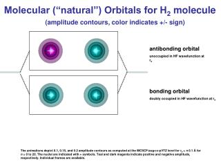
Molecular (“natural”) Orbitals for H2 molecule (amplitude contours, color indicates +/- sign) antibonding orbital unoccupied in HF wavefunction at re bonding orbital doubly occupied in HF wavefunction at re The animations depict 0.1, 0.15, and 0.2 amplitude contours as computed at the MCSCF/aug-cc-pVTZ level for re + n 0.1 Å for n = 0 to 20. The nuclei are indicated with + symbols. Teal and dark magenta indicate positive and negative amplitude, respectively. Individual frames are available.
Natural Orbitals for H2 molecule (This time plotted as Ψ along the y-axis) Animations of the amplitudes along the bond axis for the H2 bonding and antibonding (natural) orbitals.
GVB Orbitals for H2(X1Sg+) 1sR GVB orbital singly occupied for all r 2sL GVB orbital Singly occupied for all r The animations depict 0.1, 0.15, and 0.2 amplitude contours as com-puted for re + n 0.1 Å for n = 0 to 20. The nuclei are indicated with + symbols. Individual frames are available.
GVB Orbitals for H2(X1Sg+) Animations of the amplitudes along the bond axis for the H2sR and sL GVB orbitals. GVB orbitals effectively show the degree to which the atomic orbitals involved in bonding are polarized toward the other nucleus during bond formation in order to maximize electron-proton interactions. The following sequence of slides shows GVB orbitals and their overlap for H2 at various point along the potential energy curve (and animated along the entire curve on the final slide).
Transforming NOs to GVB orbitals The GVB wavefunction for H2 is the smallest subset of all the terms of the full configuration interaction wavefunction that allows for proper dissociation to H+H. Approximate GVB orbitals can be transformed from the natural orbitals of the equivalent MCSCF wavefunction using the CI vector coefficients for the 20 and 02 configurations of sbsa, which converge upon 2-½ as r as shown in the figure.
Transforming NOs to GVB orbitals MCSCF orbitals sb/sa can be transformed straightforwardly into approximate GVB orbitals sR/sL: c’1 and c’2 are renormalized CI vector coefficients The GVB overlap is: (See previous slide for plot of SRL for H2.)
Bonding in H21Σ+ – GVB model – 2.75 Å H H 1sL 1sR
Bonding in H21Σ+ – GVB model – 1.65 Å H H 1sL 1sR
Bonding in H21Σ+ – GVB model – 1.35 Å H H 1sL 1sR
Bonding in H21Σ+ – GVB model – 1.05 Å H H 1sL 1sR
Bonding in H21Σ+ – GVB model – 0.75 Å H H 1sL 1sR
Bonding in H21Σ+ – GVB model – ANIMATION H H 1sL 1sR