A Sparse Signal Reconstruction Perspective for Source Localization with Sensor Arrays
260 likes | 555 Vues
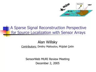
A Sparse Signal Reconstruction Perspective for Source Localization with Sensor Arrays. Müjdat Çetin Stochastic Systems Group, M.I.T. SensorWeb MURI Review Meeting September 22, 2003. Problem setup. Source localization based on passive sensor measurements

A Sparse Signal Reconstruction Perspective for Source Localization with Sensor Arrays
E N D
Presentation Transcript
A Sparse Signal Reconstruction Perspective for Source Localization with Sensor Arrays Müjdat Çetin Stochastic Systems Group, M.I.T. SensorWeb MURI Review Meeting September 22, 2003
Problem setup • Source localization based on passive sensor measurements • Context: Acoustic sensors, narrowband/wideband signals, sources in far-field/near-field, any array configuration • Issues: • Resolution • Robustness to noise • Limited observation time • Multipath, correlated sources • Model uncertainties • Our approach: View the problem as one of imaging a “source density” over the field of regard • Ill-posed inverse problem (overcomplete basis representation) • Favor sparse fields with concentrated densities
What we presented last year • Source localization framework using lp-norm-based sparsity constraints (far and near-field) • Special Quasi-Newton method for numerical solution • Preliminary experimental performance analysis • Joint source localization and self-calibration for moderate sensor location uncertainties
Data fidelity Regularizing sparsity constraint Source Localization Framework • Cost functional (notional): • Observation model: Noise Sensor measurements Array manifold matrix Unknown “source density” • Role of the regularizing constraint : • Preservation of strong features (source densities) • Preference of sparse source density field • Can resolve closely-spaced radiating sources
- - - - - - - An example • Uniform linear array with 8 sensors • Uncorrelated sources • DOAs: 50, 60 • SNR = 5 dB
Progress since then • Theoretical analysis of lp regularization • SVD-based approach for combining and summarizing multiple data samples • Optimization based on Second Order Cone (SOC) Programming • Adaptive grid refinement • Detailed performance analysis • Automatic parameter choice • Improved self-calibration procedure • Interactions • ARL: Brian Sadler, Ananthram Swami • Ohio State: Randy Moses
Theoretical analysis – setup • Basic problem: find an estimate of , where • Underdetermined -- non-uniqueness of solutions • Regularize by preferring sparse estimates • When does lp regularization yield the right solution? • Theoretical result: We can obtain the right solution by lp regularization if the actual spatial spectrum is sparse enough • Significance: • Conditions for performance guarantees and limits • Conditions for tractable solution of a combinatorial problem • Insights into the choice of regularizing constraints
Number of non-zero elements in s • Definition: A is called rank-K unambiguous if any set of K columns is linearly independent, but this is not true for K+1. • Assume A is rank-K unambiguous (for some K). • Thm. 1: • Small number of sources exact solution by l0 optimization • K ≈ number of sensors • This is a hard combinatorial optimization problem. • What can we say about more tractable formulations like l1 ? l0 uniqueness conditions • Prefer the sparsest solution: • Let (i.e. we have L point sources) • When is ?
Definition: Maximum absolute dot product of columns • Thm. 2: • Small number of sources exact solution by l1 optimization • More restrictive than the l0 condition • Can solve a combinatorial optimization problem by linear programming! l1 equivalence conditions • Consider the l1 problem: • Can we ever hope to get ?
Definition: • Thm. 3: • Small number of sources exact solution by lp optimization • Less restrictive conditions for smaller p! • Smaller p more sources can be resolved • As p0 we recover the l0 condition, namely lp(p≤1) equivalence conditions • Consider the lp problem: • How about ?
Thm. 4: (assuming rank(Y)=L) • Improves upon the single-sample l0 condition • Implication for array processing:guarantee for exact solution if # sources < # sensors ! Multi-sample l0 condition • Multiple snapshots: • Consider the l0 problem: • When is ?
Dealing with multiple snapshots • How to process multiple time samples efficiently and synergistically? • Similar problem of multiple frequency snapshots • View data as cloud of T points in a Q-dimensional subspace • Take the SVD of the data matrix • Summarize data using Q largest singular vectors • Best performance when Q is the number of sources (no catastrophic consequences in the case of other choices)
SVD-based formulation • Represent data by the largest Q singular vectors • This leads to: • Finally, we obtain the cost functional: • Natural and effective way of summarizing information contained in multiple data samples
Optimization by SOCP (for p=1) • Express the optimization problem as a second order cone program: • Solve by an efficient interior point algorithm Linear cost in auxiliary variables Quadratic, linear, and SOC constraints
Adaptive Grid Refinement • Goal: alleviate the effects of the grid, with reasonable computation • Find initial location estimates on a coarse grid • Make the grid finer around previous estimates and obtain source locations on the new grid • Iterate to required precision
Narrowband, uncorrelated sources – high SNR • DOAs: 65, 70 • SNR = 10 dB • Far-field • 200 time samples • Uniform linear array with 8 sensors
Narrowband, uncorrelated sources – low SNR • Far-field • 200 time samples • Uniform linear array with 8 sensors • DOAs: 65, 70 • SNR = 0 dB
Narrowband, correlated sources • Far-field • 200 time samples • Uniform linear array with 8 sensors • DOAs: 63, 73 • SNR = 20 dB
Robustness to limitations in data quantity Single time-sample processing • Uncorrelated sources • Uniform linear array with 8 sensors • DOAs: 43, 73 • SNR = 20 dB
Resolving many sources • 7 uncorrelated sources • Uniform linear array with 8 sensors
Estimator Variance and the CRB • Correlated sources • Uniform linear array with 8 sensors • DOAs: 43, 73 • Each point on curve average of 50 trials
Multiband/wideband case • Formulate the source localization problem in the frequency domain • Two options: • Independent processing at each frequency • Joint, coherent processing of all data • Current wideband methods are mostly incoherent • Our framework allows seamless coherent processing • Uses all data in synergy • Allows the incorporation of prior information about the temporal spectrum
Beamforming Proposed Multiple harmonics – high SNR Underlying spectrum
Beamforming MUSIC Capon’s method (MVDR) Proposed Multiband example – low SNR
Summary • Regularization-based framework for source localization with passive sensor arrays • Superior source localization performance • Superresolution • Reduced artifacts • Robustness to resource limitations • SNR • Observation time • Available aperture • Ability to handle correlated signals e.g. due to multipath effects • Adaptation to signal structures of interest to the Army (including multiband harmonic sources)
Where to from here? • Spatially-distributed sources • Extension through the use of a different overcomplete basis • Dynamic environment, mobile sources • Promising approach due to its robustness to limitations in observation time • Incorporating prior information on more complicated wideband spectra • Cyclostationary signals • Experiments with measured data (possibly through ARL)