Download
1 / 5
50 likes | 237 Vues
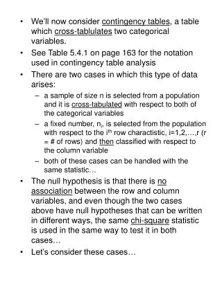
We’ll now consider contingency tables , a table which cross-tablulates two categorical variables. See Table 5.4.1 on page 163 for the notation used in contingency table analysis There are two cases in which this type of data arises:

E N D
We’ll now consider contingency tables, a table which cross-tablulates two categorical variables. • See Table 5.4.1 on page 163 for the notation used in contingency table analysis • There are two cases in which this type of data arises: • a sample of size n is selected from a population and it is cross-tabulated with respect to both of the categorical variables • a fixed number, ni, is selected from the population with respect to the ith row charactistic, i=1,2,…,r (r = # of rows) and then classified with respect to the column variable • both of these cases can be handled with the same statistic… • The null hypothesis is that there is no association between the row and column variables, and even though the two cases above have null hypotheses that can be written in different ways, the same chi-square statistic is used in the same way to test it in both cases… • Let’s consider these cases…
The expected cell proportion is and the row & column proportions are • For case 2, we define the conditional probability of column j given row i as • Case 1 null hypothesis is that the two variables are independent of each other. • Case 2 null hypothesis is that of row distribution homogeneity (i.e., for any column, the conditional probabilities from row to row are all the same) • We call both cases a test of association between the row and column variables and we use the so-called chi-square statistic to test the hypothesis.
The chi-square statistic is given as where is the expected frequency in cell (i,j). If the null hypothesis of no association between the row and column variable is true then this statistic has approximately a chi-square distribution with (r-1)(c-1) degrees of freedom. When large discrepancies exist between what we observe in the cells (nij) and what we would expect to see in the cells if the null hypothesis is true (eij) the chi-square statistic is large and leads to small p-values. • This approximation is best applied when the expected cell frequencies are 5 or more. In case this is not true, we may use a permutation test based on the chi-square statistic. • The chi-square distribution is tabulated in Table A7 on page 344 for various d.f. and various upper-tail probabilities...
Let’s look at how SAS handles contingency tables... • first consider the organization of the data: is it in “raw” form or already cross-tabulated as a contingency table? • if it’s “raw”, then PROC FREQ will put the data into a table and count the number of observations in each cell • if it’s already in tabular form, then you must use the WEIGHT statement and include a variable whose values are the counts in each cell. An example follows... • “Raw” data: data table5_4_2_raw; input trtment $ satis $ @@; datalines; pp not pp not pp somewhat pp somewhat sa somewhat sa very sa very proc freq data=table5_4_2_raw; tables trtment*satis/chisq; run; quit; • Tabular data – already cross-classified: data table5_4_2; input trtment $ satis $ count @@; datalines; pp not 2 pp somewhat 2 pp very 0 sa not 0 sa somewhat 1 sa very 2 proc freq data=table 5_4_2; tables trtment*satis/chisq; weight count; run; quit;
The above code gives the asymptotic p-value for the chi-square – to get the permutation chi-square value, use the exact chisq; statement. Or for large tables, when the computation time might be extensive, you may do random sampling of permutations as: proc freq; tables trtment*satis; exact chisq; or proc freq; tables trtment*satis; exact chisq/n=5000; • For Tuesday: Read section 5.4.1, especially considering the chi-square test in the two different formulations. Omit sections 2-4, except to do the SAS implementation of the permutation test... Do problems #8 and 9a on p. 190-191. The next set of slides finishes Chapter 5 with Fisher’s Exact Test, the Mantel-Haenszel Test, and McNemar’s Test (sections 5.5, 5.7, and 5.8) – so read ahead in these sections if you have some time. • Try these for extra practice: Injury Level None minimal minor major Seat Belt Yes 12,813 647 359 42 No 65,963 4,000 2,642 303 1 2 3 4 5 6 fair rolls 38 26 26 34 31 45 biased rolls 12 4 17 17 18 32