Continuous Random Variables

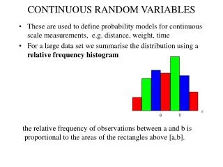
1. Continuous Random Variables

2. Consider the following table of sales, divided into intervals of 1000 units each,

3. and the relative frequency of each interval.

4. We’re going to divide the relative frequencies by the width of the cells (which here is 1000). This will make the graph have an area of 1.

5. Graph f(x) = p(x) 0.00030 0.00025 0.00020 0.00015 0.00010 0.00005 0 0 1000 2000 3000 4000 5000 6000 7000 sales The area of each bar is the frequency of the category, so the total area is 1.

6. f(x) = p(x) 0.00030 0.00025 0.00020 0.00015 0.00010 0.00005 0 0 1000 2000 3000 4000 5000 6000 7000 sales Graph Here is the frequency polygon.

7. f(x) = p(x) sales If we make the intervals 500 units instead of 1000, the graph would probably look something like this: The height of the bars increases and decreases more gradually.

8. If we made the intervals infinitesimally small, the bars and the frequency polygon would become smooth, looking something like this: This what the distribution of a continuous random variable looks like. This curve is denoted f(x) or p(x) and is called the probability density function. f(x) = p(x) sales

9. pmf versus pdf • For a discrete random variable, we had a probability mass function (pmf). • The pmf looked like a bunch of spikes, and probabilities were represented by the heights of the spikes. • For a continuous random variable, we have a probability density function (pdf). • The pdf looks like a curve, and probabilities are represented by areas under the curve.

10. f(x) = p(x) a b sales Pr(a < X < b)

11. A continuous random variable has an infinite number of possible values & the probability of any one particular value is zero.

12. If X is a continuous random variable, which of the following probabilities is largest?(Hint: This is a trick question.) • 1. Pr(a < X < b) • 2. Pr(a ≤ X < b) • 3. Pr(a < X ≤ b) • 4. Pr(a ≤ X ≤ b) They’re all equal. They differ only in whether they include the individual values a and b, and any one particular value has zero probability!

13. Properties of probability density functions (pdfs) • 1. f(x) ≥ 0 for values of x • This means that when we draw the pdf curve, while it may be on the left side of the vertical axis (have negative values of x), it can not go below the horizontal axis, where f would be negative. • Pr( - ∞ < X < ∞) = 1 • The total area under the pdf curve, which corresponds to the total probability, is 1.

14. Example • f(x) = 2 if 1 ≤ x ≤ 1.5 and • f(x) = 0 otherwise

15. Example • f(x) = 2 if 1 ≤ x ≤ 1.5 and • f(x) = 0 otherwise This function satisfies both the properties of pdfs. First, it’s never negative. Second, the total area under the curve is (1/2) (2) = 1. f(x) 2.0 0 1.0 1.5 x

16. Cumulative Distribution Function for a Continuous Random Variable • F(x) = Pr(X ≤ x) = area under the f(x) curve up to where X=x.

17. f(x) 2.0 0 1.0 1.5 x Rectangle Example: What is F(1.2)? • F(1.2) = Pr(X ≤ 1.2) • = the area under the pdf up to where x is 1.2.

18. f(x) 2.0 0 1.0 1.2 1.5 x Rectangle Example: What is F(1.2)? • F(1.2) = Pr(X ≤ 1.2) • = the area under the pdf up to where x is 1.2.

19. f(x) 2.0 0 1.0 1.2 1.5 x Rectangle Example: What is F(1.2)? • F(1.2) = Pr(X ≤ 1.2) • = the area under the pdf up to where x is 1.2. = (0.2) (2.0) = 0.4

20. The most famous distribution is the Normal or Gaussian distribution. • Its probability density function (pdf) is m is the mean of the distribution, s is the standard deviation, It is sometimes denoted N (m, s2), which means the normal distribution with a mean of m and a variance of s2.

21. m1m2m3 If you have three normal distributions with the same standard deviation (same spread), but different means (different averages), they would look like this:

22. If you had the same mean but different standard deviations, it would look like this: large standard deviation

23. If you had the same mean but different standard deviations, it would look like this: medium standard deviation large standard deviation

24. If you had the same mean but different standard deviations, it would look like this: small standard deviation middle standard deviation largest standard deviation Keep in mind that the areas are all the same, since they all equal 1.

25. Recall that if a random variable has mean m and standard deviation s, then (X-m)/s has mean 0 and standard deviation 1. • If X is normally distributed, then (X-m)/s will be standard normal, N(0,1), normal with mean 0 and variance 1. This theorem is extremely useful. It means that we don’t need to use the messy normal formula. We can standardize any normal distribution and look up probabilities in tables for the standard normal distribution.

26. Using the standard normal table is not difficult, but it takes practice to get accustomed to it. • The table in your text book gives probabilities that the standard normal (often called the Z) is between zero and a positive number, that is, Pr(0 ≤ Z ≤ a). • Some tables are set up differently, so you need to notice how a table is computed when you use it.

27. Z table: You get the integer part & the 1st decimal from the left column & the second decimal from the top row. ? 0.4957 Example: Pr(0 ≤ Z ≤ 2.63) = 0.4957 0 2.63 Z

28. Do not memorize a lot of rules. You just need to remember 2 easy facts. • The graph is symmetric about 0. • The total area under the curve is 1. 0 Z

29. Example • Pr(0 < Z < 1.85) 0 1.85 Z

30. Example • Pr(0 < Z < 1.85) = 0.4678 0.4678 0 1.85 Z

31. Example • Pr(Z < 1.85) 0.4678 0 1.85 Z

32. Example • Pr(Z < 1.85) = 0.5+ 0.4678 = 0.9678 0.5 0.4678 0 1.85 Z

33. Example • Pr(Z > 1.85) 0.4678 0 1.85 Z

34. Example • Pr(Z > 1.85) = 0.5 - 0.4678 = 0.0322 0.4678 0.0322 0 1.85 Z

35. Example • Pr(Z < -1.85) 0.4678 -1.85 0 1.85 Z

36. Example • Pr(Z < -1.85) = 0.5 - 0.4678 = 0.0322 0.4678 0.0322 -1.85 0 1.85 Z

37. Example • Pr(Z > -1.85) 0.4678 -1.85 0 1.85 Z

38. Example • Pr(Z > -1.85) = 0.5 + 0.4678 = 0.9678 0.4678 -1.85 0 1.85 Z

39. Example • Pr(-1< Z < 2) -1.00 0 2.00 Z

40. Example • Pr(-1< Z < 2) = 0.3413 + 0.4772 = 0.8185 0.3413 0.4772 -1.00 0 2.00 Z

41. Example • Pr(1< Z < 2) ? 0 1.00 2.00 Z

42. Example • Pr(1< Z < 2) = 0.4772 - 0.3413 = 0.1359 0.3413 0.4772 -1.00 0 2.00 Z

43. Example Pr(0 < Z < 5) 0 5 Z

44. Example Pr(0 < Z < 5) = 0.5000 (to 4 decimal places) 0 5 Z

45. Example Pr( Z < 5) 0 5 Z

46. Example Pr( Z < 5) = 1.0000 (to 4 decimal places) 0 5 Z

47. Example Pr( Z > 5) 0 5 Z

48. Example Pr( Z > 5) = 0.0000 (to 4 decimal places) 0 5 Z

49. Example • What is the value of k such that Pr(0 < Z < k) = 0.4750 ? 0.4750 0 k Z

50. Example • What is the value of k such that Pr(0 < Z < k) = 0.4750 ? 0.4750 0 1.96 Z