Continuous Random Variables
Continuous Random Variables. Pre-Knowledge. 1. If y = 5x 2 – 2x + 1, find . . 2. Find the turning point of the function given in question 1. 3. Solve 3x 2 – 8x + 1 = 0 giving your answers to 2 decimal places. 4. Calculate . Probability Density Function ( pdf ).

Continuous Random Variables
E N D
Presentation Transcript
Continuous Random Variables
Pre-Knowledge 1. If y = 5x2 – 2x + 1, find . 2. Find the turning point of the function given in question 1.
3. Solve 3x2 – 8x + 1 = 0 giving your answers to 2 decimal places.
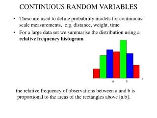
Probability Density Function (pdf) Suppose the heights of a very large number of 17 year olds was surveyed The total area under the graph is 1 and particular areas represent probabilities
Suppose the class widths were refined to 0.1m Assuming that enough data was collected the class widths could be further reduced until the ‘relative frequency polygon’ approximates to a curve. When the function ‘f(x)’ is found for the curve, it is called the probability density function, or pdf
Probability Density Function (pdf) To be a probability density function (pdf), f(x) must satisfy these basic properties: • f(x) ≥ 0 for all x, so that no probabilities are negative • ; often f(x) is only defined over a small range, in which case the integral over that range will be 1. You can find the probability that a random variable lies between x = a and x = b from the area under the curve represented by f(x) between these two points.
Example 1 (a) Show that f(x) is a probability density function where • f(x) ≥ 0 for all x, so that no probabilities are negative • f(x) is positive for all values of x • ; often f(x) is only defined over a small range, in which case the integral over that range will be 1.
Example 1 (a) Show that f(x) is a probability density function where (b) Find P(X < 4)
If f(x) is a pdf, then Example 2 gives a pdf. Draw the pdf and find P(0.5 < x < 1.3) P(0.5 < x < 1.3) f(x) 1 0 1 2 x
Example 3 (a) Find the value of k and calculate P(-1 < X < 2) (b) Find P(X = 2) • ; often f(x) is only defined over a small range, in which case the integral over that range will be 1. (a) (b) For any CONTINUOUS distribution, P(X = a) = 0 P(X = 2) = 0
Cumulative Distribution Function (cdf) In S1, the cumulative distribution function (cdf) F(x0) was defined as P(X ≤ x0) for discrete random variables. For continuous random variables, you can find the cdfby integrating the pdf. Similarly, you can find the pdf from the cdf by differentiating. Probability Density Cumulative Distribution Function (pdf) Function (cdf) f(x) F(x)
Example 4 is a pdf. Find the cumulative distribution function.
Example 5 find f(x)
Mean & Variance of a Continuous Random Variable The mean or expected value of a discrete probability distribution is defined as: μ = E(X) = Σpx For a continuous random variable: where in practice, the limits will be the interval over which f(x) is defined.
Example 6 Find E(X)
For a discrete random variable, variance, Var(X) = σ2 = E(X2) – μ2 For a continuous random variable, Example 7 Find the standard deviation for Var(X) = E(X2) – μ2
* Example 8 The continuous random variable, X, has probability density function (a) Find the value of k (b) Find the mean and variance of X. (c) Calculate i P(X > μ) ii P(X > μ + σ)
Example 9 The continuous random variable Y has probability density function Find the mean and variance of Y.
Example 10 The continuous random variable X has probability density function (a) Find the mean and variance of X. (b) Calculate i P(X > 2) ii P(|X| > σ)
Example 11 The weekly petrol consumption, in hundreds of litres, of a sales representative may be modelled by the random variable X with probability density function (a) Find the values of a and b if the mean consumption is 144 litres. (b) Find the standard deviation of the weekly petrol consumption.
Significant Values of a Continuous Random Variable The mode of a continuous random variable is the value of x for which f(x) is a maximum over the interval in which f(x) exists. This is either a stationary point, at which f ’(x) = 0, or the end value of the interval over which f(x) is defined. There may not be a mode if no single value occurs more often that any other. (Bimodal distributions do occur commonly in real life).
Example 12 Find the mode.
Example 13 Find the mode
You can use the cumulative distribution function to find the median and quartiles for a continuous random variable: If m is the median, then F(m) = 0.5 If Q1 is the lower quartile then F(Q1) = 0.25 If Q3 is the upper quartile then F(Q3) = 0.75 You can set up an appropriate algebraic equation and solve it to find the required quartile, decile or percentile.
Example 14 Find (a) the median (b) the lower and upper quartiles for X. (a) Median is when F(X)=0.5
Example 14 Find (a) the median (b) the lower and upper quartiles for X. Q3 is when F(X) = 0.75 Q1 is when F(X) = 0.25 (b)
If you were asked for the SHAPE of the distribution or the SKEW… Q2 – Q1 = 0.41 Q3 – Q2 = 0.32 Q2 – Q1 > Q3 – Q2 Negative Skew

