5. Continuous Random Variables
5. Continuous Random Variables. Delivery time. A package is to be delivered between noon and 1pm. When will it arrive?. Delivery time. A probability model. Sample space S 1 = { 0, 1, …, 59 }. equally likely outcomes . Random variable X : minute when package arrives.

5. Continuous Random Variables
E N D
Presentation Transcript
Delivery time A package is to be delivered between noon and 1pm. When will it arrive?
Delivery time A probability model Sample space S1 = {0, 1, …, 59} equally likely outcomes Random variable X: minute when package arrives X(0) = 0, X(1) = 1, …, X(59) = 59 • X(w) = w E[X] = 0⋅1/60 + … + 59⋅1/60 = 29.5
Delivery time A more precise probability model S2= {0, , , …, 1, 1 , …, 59 } equally likely outcomes • X: minute when package arrives E[X] = 29.983… 59 1 2 1 60 60 60 60
Taking precision to the limit S = the (continuous) interval[0, 60) equally likely outcomes S1 = {0, 1, …, 59} p = 1/60 S2= {0, , …, 59 } p = 1/3600 59 1 60 60 S= [0, 60) p = 0
Uncountable sample spaces In Lecture 2 we said: “The probability of an event is the sum of the probabilities of its elements” but in S = [0, 60) all elements have probability zero! To specify and calculate probabilites, we have to work with the axioms of probability
The uniform random variable Sample space S =[0, 60) Events of interest: intervals [x, y) ⊆ [0, 60) their intersections, unions, etc. P([x, y)) = (y – x)/60 Probabilities: X(w) = w Random variable:
How to do calculations You walk out of the apartment from 12:30 to 12:45. What is the probability you missed the delivery? Solution Event of interest: E = [30, 45) orE = “30 ≤ X < 45” E 60 0 P(E) = (45 – 30)/60 = 1/4
How to do calculations From 12:08 - 12:12 and 12:54 - 12:57 the doorbell wasn’t working. Event of interest: E = “8 ≤ X < 12” ∪ “54 ≤ X < 57” 60 0 P(E) = P([8, 12)) + P([54, 57)) = 4/60 + 3/60 = 7/60
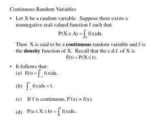
Cumulative distribution function The probability mass function doesn’t make much sense because P(X = x) = 0 for all x. Instead, we can describe X by its cumulative distribution function (c.d.f.)F: F(x) = P(X ≤ x)
Cumulative distribution functions f(x) = P(X = x) F(x) = P(X ≤ x)
Uniform random variable If X is uniform over [0, 60) then X ≤ x x 60 0 F(x) forx < 0 0 P(X ≤ x) = x/60 forx ∈[0, 60) forx > 60 1 x
Cumulative distribution functions discretec.d.f. F(x) = P(X ≤ x) p.m.f. f(x) = P(X = x) ? continuousc.d.f. F(x) = P(X ≤ x)
Discrete random variables: • p.m.f. f(x) = P(X = x) c.d.f. F(x) = P(X ≤ x) f(x) = F(x) – F(x – d) F(a) = ∑x ≤ a f(x) for small d Continuous random variables: The probability density function (p.d.f.) of a random variable with c.d.f. F(x) is • dF(x) • F(x) – F(x – d) = lim f(x) = • dx • d • d → 0
Discrete random variables: • p.m.f. f(x) = P(X = x) c.d.f. F(x) = P(X ≤ x) F(a) = ∑x ≤ a f(x) Continuous random variables: c.d.f. F(x) = P(X ≤ x) • p.d.f. f(x) = dF(x)/dx F(a) = ∫x ≤ a f(x)dx
Uniform random variable ifx < 0 0 F(x) = x/60 ifx ∈[0, 60) ifx ≥ 60 1 c.d.f. F(x) 1/60 ifx < 0 0 1/60 ifx ∈ (0, 60) dF(x)/dx = ifx > 60 0 p.d.f. f(x)
Cumulative distribution functions discretec.d.f. F(x) = P(X ≤ x) p.m.f. f(x) = P(X = x) continuousc.d.f. F(x) = P(X ≤ x) p.d.f. f(x) = dF(x)/dx
Uniform random variable A random variable X is Uniform(0, 1) if its p.d.f. is 1 ifx ∈ (0, 1) f(x) f(x) = ifx <0orx > 1 0 X A Uniform(a, b) has p.d.f. 1/(b - a) ifx ∈ (a, b) f(x) = b a ifx <aorx > b 0
Some practice A package is to be delivered between noon and 1pm. It is now 12.30 and the package is not in yet. When will it arrive?
Some practice Probability model Arrival time X is Uniform(0, 60) We want the c.d.f. of Xconditioned on X > 30: • P(X ≤ x and X > 30) • P(X ≤ x | X > 30) • = • P(X> 30) • P(30 < X ≤ x) • = • P(X> 30) • (x – 30)/60 • (x – 30)/30 • = • = • 1/2
Some practice The c.d.f. of Xconditioned on X > 30 is for x in [30, 60) G(x) = (x – 30)/30 The p.d.f. of Xconditioned on X > 30 is g(x) = dG(x)/dx = 1/30 for x in [30, 60) and 0 outside. So X conditioned onX > 30 is Uniform(30, 60).
Waiting for a friend Your friend said she’ll show up between 7 and 8 but probably around 7.30. It is now 7.30. What is the probability you have to wait past 7.45?
Waiting for a friend Probability model Let’s assume arrival time X has following p.d.f.: f(x) 1/30 x 60 0 30 We want to calculate • P(X > 45) • P(X > 45| X > 30) • = • P(X> 30)
Waiting for a friend f(x) 1/30 x 60 45 0 30 60 • = 1/2 P(X> 30) = ∫30f(x)dx 60 • = 1/8 P(X> 45) = ∫45f(x)dx • so P(X > 45| X > 30)= (1/8)/(1/2) = 1/4.
Interpretation of the p.d.f. The p.d.f. value f(x) d approximates the probability that Xin an interval of length d around x P(x –d≤ X < x) = f(x) d+ o(d) P(x ≤ X < x + d) = f(x) d+ o(d) Example 1/60 If X is uniform, then f(x) = 1/60 d P(x ≤ X < x + d) = d/60 x
Discrete versus continuous p.m.f. f(x) p.d.f. f(x) ∑x ≤ a f(x) ∫x ≤ a f(x)dx P(X ≤ a) E[X] ∑x x f(x) ∫x x f(x)dx ∑x x2 f(x) ∫x x2 f(x)dx E[X2] Var[X] E[(X – E[X])2] = E[X2] – E[X]2
Uniform random variable A random variable X is Uniform(0, 1) if its p.d.f. is 1 ifx ∈ (0, 1) f(x) = ifx <0orx > 1 0 m f(x) ∫0 f(x)dx 1 = ∫0 dx = 1 1 m +s m –s • = 1/2 • = x2/2|0 E[X] = ∫0 x f(x)dx 1 1 • = 1/3 1 • = x3/3|0 m = E[X] s = √Var[X] E[X2] = ∫0 x2 f(x)dx 1 x Var[X] = 1/3 – (1/2)2 = 1/12 √Var[X]= 1/√12 ≈ 0.289
Uniform random variable A random variable X is Uniform(a, b) if its p.d.f. is 1/(b - a) ifx ∈ (a, b) f(x) = ifx <aorx > b 0 Then E[X] = (a + b)/2 Var[X] = (b – a)2/12
Raindrops again Rain is falling on your head at an average speed of l drops/second. 2 1 How long do we wait until the next drop?
Raindrops again Probability model Time is divided into intervals of length 1/n Events Ei = “raindrop hits in interval i” have probability p = l/n and are independent X = interval of first drop X 2 1 P(X = x) • = P(E1c…Ex-1cEx) • = (1 – p)x-1p
Raindrops again X = interval of first drop X = x x-1 x T n n T = time (in seconds) of first drop (x– 1)/n ≤ T < x/n X = x means that P((x– 1)/n ≤ T < x/n) = P(X = x) • = (1 – p)x-1p • = (1 – l/n)x-1(l/n)
Raindrops again T = time (in seconds) of first drop • P((x–1)/n ≤ T < x/n) = (1 – l/n)x-1(l/n) If we set t = (x – 1)/n and d = 1/n we get • P(t ≤ T < t+ d) = (1 – d l)t/d(dl) • = dl e– (d l+ o(d l)) t/d = l e-lt P(t ≤ T < t + d) lim f(t) = • d • d → 0
The exponential random variable The p.d.f. of an Exponential(l) random variable T is le-lt ifx ≥ 0 f(t) = ifx < 0. 0 l= 1 l= 1 p.d.f. f(t) c.d.f. F(t) = P(T≤t)
The exponential random variable The c.d.f. of T is a F(a) = ∫0 le-ltdt= e-lt|0 = 1 –e-la • if a≥ 0 a What should the expected value of T be? (Hint: Rain falls at l drops/second How many seconds till the first drop?) E[T] = 1/l Var[T] = 1/l2
Poisson vs. exponential N 2 1 T Exponential(l) Poisson(l) number of events within time unit time until first event happens description • 1/l • l expectation • 1/l • l std. deviation
Memoryless property How much time between the second and third drop? 2 1 T Solution We start time when the second drop falls. What happened before is irrelevant. Then T is Exponential(l)
Expected time What is the expected time of the third drop? 2 1 T T1 T2 T3 Solution T = T1 + T2 + T3 T is not exponential but E[T]= E[T1] + E[T2] + E[T3] = 3/l

