Probability Density Function of Continuous Random Variables
Learn about probability density functions and how they are used to describe the distribution of continuous random variables. Understand the concepts of density functions, cumulative distribution functions, and uniform and exponential distributions.

Probability Density Function of Continuous Random Variables
E N D
Presentation Transcript
CIS 2033 based onDekking et al. A Modern Introduction to Probability and Statistics. 2007 Instructor Longin Jan Latecki Chapter 5: Continuous Random Variables
Probability Density Function of X A random variable (RV) X is continuous if there exists function ƒ: R R such that for any numbers a and b with a ≤ b, P(a ≤ X ≤ b) = ∫abƒ(x) dx The function ƒ has to satisfy ƒ(x) ≥ 0 for all x and ∫-∞∞ ƒ(x) dx = 1. The function ƒ is called probability density function (pdf). For both continuous and discrete RVs their probabilities map P: Ω -> [0,1], but the pmf of a discrete RV maps px: R-> [0,1] and P(X=a) =px(a), while for a continuous RV P(X=a) =P(a ≤ X ≤ a) = 0, but see next slide.
To approximate the probability density function at a point a, one must find an ε that is added and subtracted from a and then the area of the box under the curve is obtained by the following: (2ε) * ƒ(a). As ε approaches zero the area under the curve becomes more precise until one obtains an ε of zero where the area under the curve is that of a width-less box. This is shown through the following equation. P(a – ε ≤ X ≤ a +ε) = ∫a-εa+ε ƒ(x) dx ≈ 2ε*ƒ(a)
Important facts: DISCRETE NO DENSITY CONTINUOUS NO MASS BOTH CUMULATIVE DISTRIBUTION ƒ(a) = P(X ≤ a) P(a < X ≤ b) = P(X ≤ b) – P(X ≤ a) = ƒ(b) – ƒ(a) How the Distribution Function relates to the Density Function: Example for b=6.
Darts Example Suppose we want to make a probability model for an experiment: A dart hits a disc of radius r in a completely arbitrary way. We are interested in the distance X from the hitting point to the center of the disc. Since distances cannot be negative, we have F(b) = P(X ≤ b) = 0 when b < 0. Since the object hits the disc, we have F(b) = 1 when b > r. b r
Compute for the darts example the probability that 0 < X ≤ r/2, and the probability that r/2< X ≤ r. We have P(0 < X ≤ r/2) = F(r/2) − F(0) = (1/2)2 − 02 = 1/4, and P(r/2 < X ≤ r) = F(r)−F(r/2) = 1−1/4 = 3/4, no matter what the radius of the disc is.
Uniform Distribution U(α,β) • A continuous RV has a uniform distribution on the interval [α, β] if its pdf ƒ is given by ƒ(x) = 0 if x is not in [α,β] and, ƒ(x) = 1/(β-α) for α ≤ x ≤ β This simply means that any x in the interval from α to β has the same probability and anything not in the interval is zero. • The cumulative distribution is given by F(x) = 0 if x < α, F(x) = 1 if x > β, and F(x) = (x − α)/(β − α) for α ≤ x ≤ β • If U is normalized, i.e., U(0,1), then F(x)=P(U<x)=x for every x.
Exercise 5.4 John, arriving at a bus stop, just misses the bus. Suppose that he decides to walk if the (next) bus takes longer than 5 minutes to arrive. Suppose also that the time in minutes between the arrivals of buses at the bus stop is a continuous random variable with a U(4, 6) distribution. a) Let X be the time that John will wait. What is the probability that X is less than 4.5 minutes? b) What is the probability that John will walk? The pdf of U(4, 6) is given by f(x) = ½ for x in (4, 6) andf(x)=0 otherwise. a) Let X be the time until the next arrival of a bus. X has U(4; 6) distribution. Hence P(X ≤ 4.5) = ∫44.5 ½ dx = ¼ b) Since Jensen leaves when the next bus arrives after more than 5 minutes, P(X > 5) = 1 - P(X ≤ 5) = ∫45 ½ dx = ½
Exponential Distribution Exp(λ) An RV X has an exponential distribution if its pdf: ƒ(x) = λe-λx for x ≥ 0 and CDF: ƒ(a) = 1 – e-λa for a ≥ 0 The parameter λ is the inverse of the expected value of X, i.e., E(X)= 1/ λ or λ=1/E(X). If X is time in minutes, then λ is a frequency measured in min-1. For example, if arrivals occur every half a minute on average, then E(X)=0.5 and λ=2, saying that they occur with a frequency (arrival rate) of 2 arrivals per minute. This λ has the same meaning as the parameter of Poisson distribution. Intuitively: a continuous version of the geometric distribution.
ƒ(x) = λe-λx for x ≥ 0 ƒ(a) = 1 – e-λa for a ≥ 0 If waiting time is unknown, it is often appropriate to think of it as a random variable having an exponential distribution. How much time will elapse before an earthquake occurs in a given region? How long do we need to wait before a customer enters our shop? How long will it take before a call center receives the next phone call? How long will a piece of machinery work without breaking down? Questions such as these are often answered in probabilistic terms using the exponential distribution. All these questions concern the time we need to wait before a certain event occurs.
Roughly speaking, the time we need to wait before an event occurs has an exponential distribution if the probability that the event occurs during a certain time interval is proportional to the length of that time interval. More precisely, X has an exponential distribution if the conditional probability is approximately proportional to the length Δt of the time interval [t, t+ Δt] for any time instant t . In most practical situations this property is very realistic and this is the reason why the exponential distribution is so widely used to model waiting times. From: http://www.statlect.com/ucdexp1.htm
Quick exercise 5.4 A study of the response time of a certain computer system yields that the response time in seconds has an exponentially distributed time with parameter 0.25. What is the probability that the response time exceeds 5 seconds? If X is the response time, then we ask for P(X >5). This equals P(X > 5) = 1 - P(X ≤ 5) = 1 - ƒ(a) = 1 – (1 – e-0.25*5 ) = e−1.25 = 0.2865 We used here a simple but important fact: P(X > a) = 1 - P(X ≤ a) for any real number a. This is so, since P(X ≤ a) + P(X > a) = 1, which follows from the second axiom of the def. of probability.
Example 4.5. (Baron) • Jobs are sent to a printer at an average rate of 3 jobs per hour. • (a) What is the expected time between jobs? • What is the probability that the next job is sent within 5 minutes? • Solution. • Job arrivals represent rare events, thus the time T between them is exponential with the given parameter λ = 3 hrs−1 (jobs per hour). • (a) E(T) = 1/λ = 1/3 hours or 20 minutes between jobs; • (b) Convert to the same measurement unit: 5 min = (1/12) hrs. Then
Exponential Distribution Exp(λ) The exponential distribution satisfies the memoryless property, i.e., if X has an exponential distribution, then for all s, t > 0, P(X >s + t |X >s) = P(X >t) This simply means that s becomes the origin for t. Proof: P(X > s + t | x > s) = P(x > s + t)/P(x>s) = (e-λ(s+t))/(e-λs) =e-λt= P(X > t)
Pareto Distribution Par(α) Used for estimating real-life situations such as • the number of people whose income exceeded level x, • city sizes, earthquake rupture areas, insurance claims, and sizes of commercial companies. A continuous random variable has a Pareto distribution with parameter α > 0 if its probability density function ƒ is given by ƒ(x) = 0 if x < 1 and for x ≥ 1
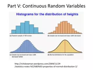
Normal Distribution N(μ,σ2) Normal Distribution (Gaussian Distribution) with parameters μ and σ2 > 0 if its probability density function ƒ is given by for -∞ < x < ∞ where μ = mean and σ2 = standard deviation Distribution function is given by: for -∞ < a < ∞ However, since ƒ does not have an antiderivative there is no explicit expression for Ƒ. Standard normal distribution N(0,1) is given as follows, and the distribution function is obtained similarly denoted by capital phi. for -∞ < x < ∞
Quantiles Portions of the whole which increase from left to right, meaning the 0th percentile is on the left hand side and the 100th percentile is on the right side. Let X be a continuous random variable and let p be a number between 0 and 1. The pth quantile or 100pth percentile of the distribution of X is the smallest number qp such that Ƒ(qp) = P(X ≤ qp) = p The median is the 50th percentile
Ƒ(qp) = P(X ≤ qp) = p For continuous random variables qp is often easy to determine. If F is strictly increasing from 0 to 1 on some interval (which may be infinite to one or both sides), then qp = Finv(p), where Finv is the inverse of F.
What is the median of the U(2, 7) distribution? pdf The median is the number q0.5 = Finv(0.5). You either see directly that half of the mass is in the middle of the interval, hence q0.5 = (2+7)/2 = 4.5, or you solve with the distribution function: F(qp) = P(X ≤ qp) = p = 0.5 F(q) = 0.5 and F(x) = (x − α)/(β − α) CDF 0.5
Find the 0.9th quantile of a standard normal distribution. F(qp) = P(X ≤ qp) = p = 0.9 The smallest a such that F(a) = 0.9 => a = Finv(0.9) Matlab: a = norminv(0.9,0,1) => a =1.2816

