Download
1 / 33
330 likes | 577 Vues
Chapter 6 Random Variables I can find the probability of a discrete random variable. 6.1a Discrete and Continuous Random Variables and Expected Value. Discrete and Continuous Random Variables. A random variable is a quantity whose value changes. Discrete Random Variable.

E N D
Chapter 6Random VariablesI can find the probability of a discrete random variable. 6.1a Discrete and Continuous Random Variables and Expected Value
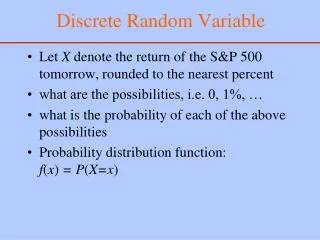
Discrete and Continuous Random Variables • A random variableis a quantity whose value changes.
Discrete Random Variable A discrete random variable is a variable whose value is obtained by counting. • number of students present • number of red marbles in a jar • number of heads when flipping three coins • students’ grade level
Probability Distribution • The probability distribution of X lists the values and their probabilities. • Value of X: x1, x2, x3, … , xk • Probability: p1, p2 , p3 , … , pk • To find the probability of event pi, add up the probabilities of the xi that make up that event.
Example: Getting Good Grades A teacher gives the following grades: • 15% A’s and D’s, 30% B’s, C’s; 10% F’s • on a 4 point scale (A=4). • Chose a student at random and find the probability they get a B or better.
Here is the distribution of X: Grade: 0 1 2 3 4 Prob: .10 .15 .30 .30 .15 • P(get a B or better) s/a P(grade 3 or 4): • P(X=3) + P(X=4) • = 0.30 + 0.15 • = 0.45
Probability Histograms • Height of each bar is the probability • Heights add up to 1 • Prob. of Benfords Law vs. random digits
Example: Tossing Coins a. Find the probability distribution of the discrete random variable X that counts the # heads in 4 tosses of a coin. • Assume: fair coin, independence • Determine the # of possible outcomes
X = # heads • X = 0, X = 1, X = 2, X = 3, X = 4
b. Find each probability P(X=0) = 1/16 = 0.0625 P(X=1) = P(X=2) = P(X=3) = P(X=4) = • Do they add up to 1? • Yes, so legitimate distribution.
c. Describe the probability histogram. • It is exactly symmetric. • It is the idealization of the relative frequency distribution of the number of heads after many tosses of four coins.
d. What is the prob. of tossing at least 2 heads? • P(X ≥ 2) = P(X=2) + P(X=3) + P(X=4) • = 0.375 + 0.25 + 0.0625 = 0.6875
e. What is the prob. of tossing at least 1 head? • P(X ≥ 1): use the complement rule • = 1 – P(X=0) • = 1 – 0.0625 = 0.9375
Exercise: Roll of the Die If a carefully made die is rolled once, is it reasonable to assign probability 1/6 to each of the six faces? • a. What is the probability of rolling a number less than 3?
P(X<3) = P(X=1) + P(X=2) = 1/6 + 1/6 = 2/6 = 1/3 = 0.33
Exercise: Three Children • A couple plans to have three children. There are 8 possible arrangements of girls and boys. • For example, GGB. All 8 arrangements are approximately equally likely.
a. Write down all 8 arrangements of the sexes of three children. What is the probability of any one of these arrangements? • BBB, BBG, BGB, GBB, GGB, GBG, BGG, GGG • Each has probability of 1/8
b. Let X be the number of girls the couple has. • BBB, BBG, BGB, GBB, GGB, GBG, BGG, GGG • What is the probability that X = 2? • 3/8 = 0.375
c. Starting from your work in (a), find the distribution of X. • That is, what values can X take, and what are the probabilities of each value? • (Hint: make a table.)
Review of Probability • The probability of a random variable is an idealized relative frequency distribution. • Histograms and density curves are pictures of the distributions of data. • When describing data, we moved from graphs to numerical summaries such as means and standard deviations.
The Mean of a Random Variable Now we will make the same move to expand our description of the distribution of random variables. • The meanof a discrete random variable, X, is its weighted average. • Each value of X is weighted by its probability. Not all outcomes need to be equally likely.
Example: Tri-Sate Pick 3 • You pick a 3 digit number. If your number is chosen you win $500. There are 1000, 3 digit numbers. Each pick costs $1.
Taking X to be the amount your ticket pays you, the probability distribution is: • Payoff X: $0 $500 • Probability: 0.999 0.001 Find your average Payoff. • Normal “average”: (0 + 500) /2 =$250
Are the outcomes equally likely? The long run weighted average is: • = 500(1/1000) + 0(999/1000) = $ 0.50 Conclusion: • In the long run, the state keeps ½ of what you wager.
Expected Value(μx) (The long run average outcome) • We do not expect one observation to be close to its expected value. • μx : probabilities add to 1
Mean of a Discrete Random Variable • The mean of a discrete random variable, X, is its weighted average. Each value of X is weighted by its probability. • To find the mean of X, multiply each value of X by its probability, then add all the products.
Example: Benford’s Law Recall: If the digits in a set of data appear “at random,” the nine possible digits 1 to 9 all have the same probability each being 1/9. • The mean of the distribution is: μx= 1(1/9) + 2(1/9) + … + 9(1/9) = 45(1/9) = 5
But, if the data obey Benford’s law, the distribution of the first digit V is: • Find the μv: =
= 3.441 • The means reflect the greater probability of smaller digits under Benfors’s law.
Histograms of μx and μv • We can’t locate the mean of a right skew distribution by eye – calculation is needed.