Discrete Random Variables
Discrete random variables associate numerical values with outcomes in experiments, such as rolling dice. This guide covers key concepts, including how to define probability distributions, expected values, and variance, as well as their applications in statistical analysis. By examining discrete random variables, such as the sum of dice rolls or the radius of circles, we can grasp essential ideas that underpin probability theory. Understanding these foundational elements allows for better predictions and inferences about broader populations.


Discrete Random Variables
E N D
Presentation Transcript
:9101112 Numerical Outcomes • Consider associating a numerical value with each sample point in a sample space. • (1,1) (1,2) (1,3) (1,4) (1,5) (1,6) • (2,1) (2,2) (2,3) (2,4) (2,5) (2,6) • (3,1) (3,2) (3,3) (3,4) (3,5) (3,6) • (4,1) (4,2) (4,3) (4,4) (4,5) (4,6) • (5,1) (5,2) (5,3) (5,4) (5,5) (5,6)(6,1) (6,2) (6,3) (6,4) (6,5) (6,6) • For example, associate each roll of 2 dice with the sum of their faces.
Random Variable • A real-valued functionwhose domain is the sample space Sis a random variable for the experiment. :(3, 6)(4, 6)(5, 5)(6, 4)(5, 6) : : 9101112 Y S • We refer to values of the random variable as events. For example, {Y = 9}, {Y = 10}, etc.
Probability Y = y • The probability of an event, such as {Y = 9} is denoted P(Y = 9). • In general, for a real number y, the probability of {Y = y} is denoted P(Y = y), or simply, p( y). • P(Y = y) is the sum of probabilities for sample points which are assigned the value y. • When rolling two dice, P(Y = 10) = P({(4, 6)}) + P({(5, 5)}) + P({(6, 4)}) = 1/36 + 1/36 + 1/36 = 3/36
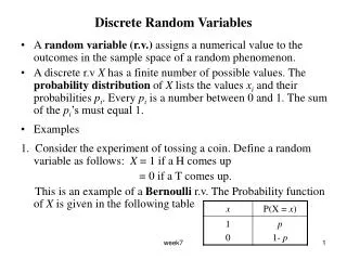
Discrete Random Variable • A discrete random variable is a random variable that only assumes a finite (or countably infinite) number of distinct values. • For an experiment whose sample points are associated with the integers or a subset of integers, the random variable is discrete. • For an experiment whose sample points are associated with the reals or an interval of real numbers, the random variable is not discrete.(Chapter 4 considers “continuous random variables”.)
“Towards Statistics” • Studying probability, we learn about certain types of random variables that occur frequently in practice and their probability distributions. Knowledge about the probabilities of these common random variables may help us make appropriate inferences about a population. (page 84). • Remember, our theoretical models represent the distribution that may be expected but may differ from the actual frequencies resulting from an experiment. (page 87)
Probability Distribution • A probability distribution describes the probability for each value of the random variable. y p(y)2 1/363 2/364 3/365 4/366 5/367 6/368 5/369 4/3610 3/3611 2/3612 1/36 Presented as a table, formula, or graph.
Probability Distribution • For a probability distribution: y p(y)2 1/363 2/364 3/365 4/366 5/367 6/368 5/369 4/3610 3/3611 2/3612 1/36 = 1.0 Here we may take the sum just over those values of yfor which p(y) is non-zero.
Expected Value • The “long run theoretical average” • For a discrete R.V. with probability function p(y), define the expected value of Y as: • In a statistical context, E(Y) is referred to as the mean and so E(Y) and m are interchangeable.
An average circle? • Suppose a class has cut some circles out of construction paper, as described below. Radius(inches) frequency 3 150 4 200 6 125 Let radius be the random variable, R.Compute E(R).
Function of a Random Variable • Suppose g(Y) is a real-valued function of a discrete random variable Y. s y g(y) S g(Y) Y • It follows g(Y) is also a random variable with expected value
Expected Circumference • Consider the function C = 2pR. • C is a function of a random variable, and so C is also a random variable. Radius(inches) circumference frequency 3 6p 150 4 8p 200 6 12p 125 • Compute the expected value, E(C).
For a constant multiple… • Of course, a constant multiple may be factored out of the sum • Thus, for our circles, E(C) = E(2pR) = 2pE(R).
For a constant function… • In particular, if g(y) = c for all y in Y, then E[g(Y)] = E(c) = c.
For sums of variables… • Also, if g1(Y) and g2(Y) are both functions of the random variable Y, then
All together now… • So, when working with expected values, we have • Thus, for a linear combination Z = c g(Y) + b,where c and b are constants:
Variance, V(Y) • For a discrete R.V. with probability function p(y), define the variance of Y as: • Here, we use V(Y) and s2 interchangeably to denote the variance. • As previously, the positive square root of the variance is the standard deviation of Y.
Computing V(Y) • Based on our definition of the variance of Y • And applying our rules for expected value, we find variance may be expressed as (as the mean is a constant)
“Moments and Mass” • Note the probability function p(y) for a discrete random variable is also called a “probability mass function”. • The expected values E(Y) and E(Y2) are called the first and second moments, respectively. Did you compute mass and moments in Calculus?
Variance of R? • For our collection of circles, determine the variance of the random variable R Radius(inches) frequency 3 150 4 200 6 125 It’s your choice. Which formula is easier? or
It can be shown that Variance of C? • For our collection of circles, determine the variance, Radius(inches) circumference frequency 3 6p 150 4 8p 200 6 12p 125