C4: DISCRETE RANDOM VARIABLES
C4: DISCRETE RANDOM VARIABLES. CIS 2033 based on Dekking et al. A Modern Introduction to Probability and Statistics . 2007 Longin Jan Latecki. Discrete Random Variables. Discrete random variables (RVs) are obtained by counting and have sample spaces

C4: DISCRETE RANDOM VARIABLES
E N D
Presentation Transcript
C4: DISCRETE RANDOM VARIABLES CIS 2033 based on Dekking et al. A Modern Introduction to Probability and Statistics. 2007 Longin Jan Latecki
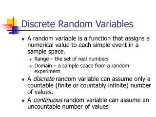
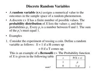
Discrete Random Variables Discrete random variables (RVs) are obtained by counting and have sample spaces which are countable. The values that represent each outcome are usually integers. Random variables are denoted by capital letters. For example, a RV X: is the number of times that we flip a coin until H comes up The possible outcomes are denoted by lower case letters: a=1, a=2, a=3...
Example from Section 4.1 RV S is the sum of two independent throws with a die. The sample space is Ω = {(ω1, ω2) : ω1, ω2 ∈ {1, 2, . . . , 6} } = {(1, 1), (1, 2), . . . , (1, 6), (2, 1), . . . , (6, 5), (6, 6)}. Hence the RV S is the function S : Ω → R, given by S( ω1, ω2 ) = ω1 + ω2 for (ω1, ω2) ∈ Ω Let {S = k} = {(ω1, ω2) ∈ Ω : S( ω1, ω2) = k }. We denote the probability of the event {S = k} by P(S = k) , although formally we should write P({S = k}) instead of P(S = k). In our example, S attains only the values k = 2, 3, . . . , 12 with positive probability. For example, P(S = 2) = P((1, 1) ) = 1/36, P(S = 3) = P({(1, 2), (2, 1)}) = 2/36, while P(S = 13) = P( ∅) = 0, because 13 is an impossible outcome. Another example of a RV is the function M : Ω → R, given by M( ω1, ω2) =max{ω1, ω2} for (ω1, ω2) ∈ Ω.
Probability Mass Function The probability mass function (pmf) of a discrete random variable maps each possible outcome in the sample space to it's corresponding probability. As an example we give the probability mass function p of M The sum of the probabilities of all possible outcomes will always be equal to 1.
Example 3.1. (Baron) • Consider an experiment of tossing 3 fair coins and counting the number of heads. • Let X be the number of heads . Prior to an experiment, its value is not known. All we can say is that X has to be an integer between 0 and 3. We can compute probabilities Hence X is a discrete RV with the following pmf: We know that X as a RV is a function M : Ω → R. What is Ω here?
Probability Distribution Function The distribution function of a random variable X, also referred to as the cumulative distribution function (CDF) yields the probability that X will take a value less than or equal to a. Hence, the value of F(a) is equal to the sum of all probabilities of outcomes less than or equal to a: If we are given a CDF, we can get the pmf with the following formula: for some sufficiently small ε>0.
Graphs of pmf and CDF Cumulative Distribution Function Probability Mass Function
Example 3.3 (Baron) (Errors in independent modules) • A program consists of two modules. The number of errors X1 in the first module has the pmf P1(x), and the number of errors X2 in the second module has the pmf P2(x), independently of X1 given by the table. Find the pmf and cdf of Y = X1 + X2, the total number of errors. • Solution. We break the problem into steps. First, determine all possible values of Y, then compute the probability of each value. Clearly, the number of errors Y is an integer that can be as low as 0 + 0 = 0 and as high as 3 + 2 = 5. Since P2(3) = 0, the second module has at most 2 errors. pmf CDF Check:
Bernoulli Distribution • The Bernoulli distribution is used to model an experiment with only two outcomes, success and failure. The parameter p is the chance for success. • An example is flipping a coin, where “heads” may be success and “tails” may be failure.
Binomial Distribution • The Binomial Distribution represents multiple Bernoulli trials. The parameter n is the number of trials, and the parameter p is the probability of success as in the Bernoulli distribution. • P(X=k) is the probability of k successful outcomes in n trials.
Probability mass function and distribution function of the Bin(10, 1/4 ) distribution. See Section 4.3
Geometric Distribution • A geometric distribution gives information about the probability of success after k attempts. The parameter p is the probability of success on the kth try. • This means that all previous k-1 tries failed • An example of this would be finding the probability that you will hit a bullseye with a dart on your kth toss.
Example:If we flip a coin until it lands on heads, the random variable X of the experiment is the number of times the coin needs to be flipped until heads came up. If the chance of landing on heads is p, the chance of landing on tails is 1-p. Therefore:P(X=1) = p. P(X=2) = (1 – p)1p. P(X=3) = (1-p)2pand in general P(X=n) = (1-p)n-1p We had a geometric distribution in Ch. 2: The pmf and CDFfor p=1/4, i.e., of Geo(1/4)


