Continuous Random Variables and Reliability Analysis
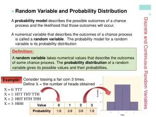
In the Name of the Most High . Continuous Random Variables and Reliability Analysis. Behzad Akbari Spring 2009 Tarbiat Modares University. These slides are based on the slides of Prof. K.S. Trivedi (Duke University). Definitions. Distribution function:

Continuous Random Variables and Reliability Analysis
E N D
Presentation Transcript
In the Name of the Most High Continuous Random Variables and Reliability Analysis Behzad Akbari Spring 2009 Tarbiat Modares University These slides are based on the slides of Prof. K.S. Trivedi (Duke University)
Definitions • Distribution function: • If FX(x) is a continuous function of x, then X is a continuous random variable. • FX(x): discrete in x Discrete rv’s
Definitions (Continued) Equivalence: • CDF (cumulative distribution function) • PDF (probability distribution function) • Distribution function • FX(x) or FX(t) or F(t)
Probability Density Function (pdf) • X : continuous rv, then, • pdf properties:
Definitions(Continued) • Equivalence: pdf • probability density function • density function • density • f(t) = For a non-negative random variable
Exponential Distribution • Arises commonly in reliability & queuing theory. • A non-negative random variable • It exhibits memoryless (Markov) property. • Related to (the discrete) Poisson distribution • Interarrival time between two IP packets (or voice calls) • Time to failure, time to repair etc. • Mathematically (CDF and pdf, respectively):
CDF of exponentially distributed random variable with = 0.0001 F(t) 12500 25000 37500 50000 t
Memoryless property • Assume X > t. We have observed that the component has not failed until time t. • Let Y = X - t , the remaining (residual) lifetime • The distribution of the remaining life, Y, does not depend on how long the component has been operating. Distribution of Y is identical to that of X.
Memoryless property • Assume X > t. We have observed that the component has not failed until time t. • Let Y = X - t , the remaining (residual) lifetime
Memoryless property (Continued) • Thus Gt(y) is independent of t and is identical to the original exponential distribution of X. • The distribution of the remaining life does not depend on how long the component has been operating.
Reliability as a Function of Time • Reliability R(t): failure occurs after time ‘t’. Let X be the lifetime of a component subject to failures. • Let N0: total no. of components (fixed); Ns(t): surviving ones; Nf(t): failed oneby time t.
Definitions (Continued) Equivalence: • Reliability • Complementary distribution function • Survivor function • R(t) = 1 -F(t)
Failure Rate or Hazard Rate • Instantaneous failure rate: h(t) (#failures/10k hrs) • Let the rv X be EXP( λ). Then, • Using simple calculus the following applies to any rv,
Hazard Rate and the pdf h(t) t = Conditional Prob. system will fail in (t, t + t) given that it has survived until time t f(t) t = Unconditional Prob. System will fail in (t, t + t) • Difference between: • probability that someone will die between 90 and 91, given that he lives to 90 • probability that someone will die between 90 and 91
Weibull Distribution • Frequently used to model fatigue failure, ball bearing failure etc. (very long tails) • Reliability: • Weibull distribution is capable of modeling DFR (α < 1), CFR (α = 1) and IFR (α >1) behavior. • α is called the shape parameter and is the scale parameter
Failure rate of the weibull distribution with various values of and = 1 5.0 1.0 2.0 3.0 4.0
Infant Mortality Effects in System Modeling • Bathtub curves • Early-life period • Steady-state period • Wear out period • Failure rate models
Until now we assumed that failure rate of equipment is time (age) independent. In real-life, variation as per the bathtub shape has been observed Bathtub Curve Failure Rate l(t) Infant Mortality (Early Life Failures) Wear out Steady State Operating Time
Early-life Period • Also called infant mortality phase or reliability growth phase • Caused by undetected hardware/software defects that are being fixed resulting in reliability growth • Can cause significant prediction errors if steady-state failure rates are used • Availability models can be constructed and solved to include this effect • Weibull Model can be used
Steady-state Period • Failure rate much lower than in early-life period • Either constant (age independent) or slowly varying failure rate • Failures caused by environmental shocks • Arrival process of environmental shocks can be assumed to be a Poisson process • Hence time between two shocks has the exponential distribution
Failure rate increases rapidly with age Properly qualified electronic hardware do not exhibit wear out failure during its intended service life (Motorola) Applicable for mechanical and other systems Weibull Failure Model can be used Wear out Period
Bathtub curve DFR phase: Initial design, constant bug fixes CFR phase: Normal operational phase IFR phase: Aging behavior h(t) (burn-in-period) (wear-out-phase) CFR (useful life) DFR IFR t Increasing fail. rate Decreasing failure rate
We use a truncated Weibull Model Infant mortality phase modeled by DFR Weibull and the steady-state phase by the exponential Failure Rate Models 7 6 5 4 3 2 1 0 Failure-Rate Multiplier 0 2,190 4,380 6,570 8,760 10,950 13,140 15,330 17,520 Operating Times (hrs)
This model has the form: where: steady-state failure rate is the Weibull shape parameter Failure rate multiplier = Failure Rate Models (cont.)
There are several ways to incorporate time dependent failure rates in availability models The easiest way is to approximate a continuous function by a decreasing step function Failure Rate Models (cont.) 7 6 5 4 3 2 1 0 Failure-Rate Multiplier 0 2,190 4,380 6,570 8,760 10,950 13,140 15,330 17,520 Operating Times (hrs)
Failure Rate Models (cont.) • Here the discrete failure-rate model is defined by:
Uniform Random Variable • U(a,b) pdf constant over the (a,b) interval and CDF is the ramp function
Uniform distribution • The distribution function is given by: 0 , x < a, F(x)= , a < x < b 1 , x > b. {
HypoExponential • HypoExp: multiple Exp stages in series. • 2-stage HypoExp denoted as HYPO(λ1, λ2). The density, distribution and hazard rate function are: • HypoExp results in IFR: 0 min(λ1, λ2) • Disk service time may be modeled as a 3-stage Hypoexponential as the overall time is the sum of the seek, the latency and the transfer time
Erlang Distribution • Special case of HypoExp: All stages have same rate.
Gamma Random Variable • Gamma density function is, • Gamma distribution can capture all three failure modes, viz. DFR, CFR and IFR. • α = 1: CFR • α <1 : DFR • α >1 : IFR
HyperExponential Distribution • Hypo or Erlang Sequential Exp( ) stages. • Alternate Exp( ) stages HyperExponential. • CPU service time may be modeled as HyperExp
Gaussian (Normal) Distribution • Bell shaped pdf • Central Limit Theorem: mean of a large number of mutually independent rv’s (having arbitrary distributions) starts following Normal distribution as n • μ: mean, σ: std. deviation, σ2: variance (N(μ, σ2)) • μ and σ completely describe the statistics. This is significant in statistical estimation/signal processing/communication theory etc.
Normal Distribution (contd.) • N(0,1) is called normalized Guassian. • N(0,1) is symmetric i.e. • f(x)=f(-x) • F(z) = 1-F(z). • Failure rate h(t) follows IFR behavior. • Hence, N( ) is suitable for modeling long-term wear or aging related failure phenomena.
Order Statistics: KofN X1 ,X2 ,..., Xn iid (independent and identically distributed) random variables with a common distribution function F(). Let Y1 ,Y2 ,...,Yn be random variables obtained by permuting the set X1 ,X2 ,..., Xn so as to be in increasing order. To be specific: Y1 = min{X1 ,X2 ,..., Xn} and Yn = max{X1 ,X2 ,..., Xn}
Order Statistics: KofN(Continued) • The random variable Yk is called the k-th ORDER STATISTIC. • If Xi is the lifetime of the i-th component in a system of n components. Then: • Y1will be the overall series system lifetime. • Yn will denote the lifetime of a parallel system. • Yn-k+1 will be the lifetime of an k-out-of-n system.
Order Statistics: KofN (Continued) To derive the distribution function of Yk, we note that the probability that exactly j of the Xi's lie in (- ,y] and (n-j) lie in (y, ) is:
Applications of order statistics • Reliability of a k out of n system • Series system: • Parallel system: • Minimum of n EXP random variables is special case of Y1= min{X1,…,Xn} where Xi~EXP(i) Y1~EXP( i) • This is not true (that is EXP dist.) for the parallel case
Triple Modular Redundancy (TMR) R(t) • An interesting case of order statistics occurs when we consider the Triple Modular Redundant (TMR) system (n = 3 and k = 2). Y2 then denotes the time until the second component fails. We get: Voter R(t) R(t)
TMR (Continued) • Assuming that the reliability of a single component is given by, we get:
TMR (Continued) • In the following figure, we have plotted RTMR(t) vs t as well as R(t) vs t.
EXP() EXP() Cold standby (dynamic redundancy) X Y Lifetime of Active EXP() Lifetime of Spare EXP() Total lifetime 2-Stage Erlang Assumptions: Detection & Switching perfect; spare does not fail
Sum of RVs: Standby Redundancy • Two independent components, X and Y • Series system (Z=min(X,Y)) • Parallel System (Z=max(X,Y)) • Cold standby: the life time Z=X+Y
Sum of Random Variables • Z = Φ(X, Y) ((X, Y) may not be independent) • For the special case, Z = X + Y • The resulting pdf is (assuming independence), • Convolution integral (modify for the non-negative case)
Convolution (non-negative case) Z = X + Y, X & Y are independent random variables (in this case, non-negative) • The above integral is often called the convolution of fX and fY. Thus the density of the sum of two non-negative independent, continuous random variables is the convolution of the individual densities.
Cold standby derivation • X and Y are both EXP() and independent. • Then
Cold standby derivation(Continued) • Z is two-stage Erlang Distributed