1. Probability and Statistics for Computer ScientistsSecond Edition, By: Michael BaronChapter 4: Continuous DistributionsCIS 2033. Computational Probability and Statistics Pei Wang

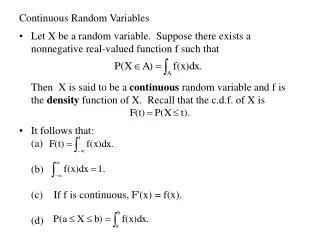
2. Continuous random variables A continuous random variable can take any value in an interval, open or closed, so it has innumerable values Examples: the height or weight of a chair For such a variable X, the probability assigned to an exact value P(X = a) is always zero, though the probability for it to fall into interval [a, b], that is, P(a ≤ X ≤ b), can be positive

3. Probability density function One way to get P(a ≤ X ≤ b): to integrate the probability density function of X

4. Probability density function (2) P(a ≤ X ≤ b) = P(a < X ≤ b) = P(a < X < b) = P(a ≤ X < b)

5. Probability density function (3)

6. Cumulative distribution function Another way to get P(a ≤ X ≤ b): P(a < X ≤ b) = P(X ≤ b) – P(X ≤ a) = F(b) – F(a) A discrete random variable has no pdf f(x), a continuous random variable has no pmf p(x), but both have a cdf F(x)

7. Review: derivative and integral • Derivatives of elementary functions power, exponential and logarithmic functions • Rules for finding the derivative combined functions • Integral as antiderivative e.g., for power function xt dx= (bt+1 – at+1) / (t+1) when t ≠ -1 dx= dx= ln(b) –ln(a)

8. Pmf p(x) versus pdf f(x)

9. Example 4.1 (1)

10. Example 4.1 (2)

11. Joint distributions: continuous

12. Joint distributions: continuous (2)

13. Pmf p(x) versus pdf f(x): joint

14. Expectation of continuous variable

15. p(x) vs. f(x): E[X] and Var(X)

16. Example 4.2

17. Uniform distribution The distribution function F of a random variable that has a U(α, β) distribution is given by      F(x) = 0 if x < α    F(x) = (x − α) / (β − α) if α ≤ x ≤ β F(x) = 1 if x > β  

18. Uniform distribution (2)

19. Uniform distribution (3) U(0, 1) is called Standard Uniform distribution Its density is f(x) = 1 for 0 < x < 1 If X is U(a, b), then Y = (X – a) / (b – a) is U(0, 1)

20. Exponential distribution When the number of events is Poisson, the time between events is exponential E[X] = 1 / λ, Var(X) = 1 / λ2

21. Exponential distribution (2)

22. Gamma distribution When a certain process consists of α independent steps, and each step takes Exponential(λ) amount of time, then the total time has a Gamma distribution with parameters α and λ

23. Gamma distribution (2)

24. Normal distribution Normal (Gaussian) distribution N(μ,2) is often used as a model for physical variables like weight, height, temperature, or examination grade.

25. Normal distribution (2)

26. Normal distribution (3) Bin(n, p) ≈ N(np, np(1 – p)) when n is large and p is moderate. Example: bean machine N(0, 1) is called Standard Normal distribution, written as φ(x). See Table A4.

27. Central Limit Theorem The Central Limit Theorem (CLT) states that, in most situations, when many independent random variables of the same type are added, their properly normalized sum tends toward a normal distribution, even if the original variables themselves are not normally distributed, that is, they can have any distribution

28. Central Limit Theorem (2) Let X1, X2,… be independent random variables with the same expectation μ = E(Xi) and the same standard deviation s = Std(Xi), and let As n → ∞, the standardized sum converges in distribution to a Standard Normal random variable for all z

29. Central Limit Theorem (3)