Continuous Random Variables
Continuous Random Variables. Section 7.1.2. Starter 7.1.2. A 9-sided die has three faces that show 1, two faces that show 2, and one face each showing 3, 4, 5, 6. Let X be the number that shows face-up. Draw the PDF histogram of X. Objectives.

Continuous Random Variables
E N D
Presentation Transcript
Continuous Random Variables Section 7.1.2
Starter 7.1.2 • A 9-sided die has three faces that show 1, two faces that show 2, and one face each showing 3, 4, 5, 6. • Let X be the number that shows face-up. • Draw the PDF histogram of X.
Objectives • Display the PDF of a continuous random variable as a density curve. • Find the probability that a continuous random variable is within a specified interval by finding the area under a density curve. California Standard 4.0 Students understand the notion of a continuous random variableand can interpret the probability of an outcome as the area of a region under the graph of the probability density function associated with the random variable.
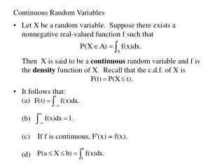
Definitions • A random variable is a variable whose value is the numerical outcome of a random event. • A continuous random variable can take on ANY value within a specified interval. • The probability distribution function (PDF) of a continuous r.v. is represented by a density curve.
The Probability of a Continuous R.V. • Consider the spinner on the overhead projector. • When I spin it, what is the probability that it lands on a number between .3 and .5? • What is the probability that it lands on a number between 0 and 1? • Draw a density curve that shows the possible outcomes and probabilities. • You are drawing the PDF of X
The Density Curve of a Continuous R.V. • For the spinner, you drew a rectangle whose X values go from 0 to 1 and whose Y values are always exactly 1. • Recall that this is called a uniform distribution • The probability of an event is the area under the curve and above the range of X values that make up the event. • So P(.3 x .5) is 0.2 because that is the area under the curve above that range of x
The Probability of One Exact Outcome • When I spin the spinner, what is the probability of hitting 0.3 exactly? • In notation: evaluate P(X = 3) • No matter how close I come, a really precise measurement will show some error. • Example: How tall are you EXACTLY? • Example: Watch the TI try to match an exact number with its random number generator. • Run program CONTRV • Conclusion: The probability of any exact outcome is always zero! • Note that the area above a point (like x = .3) is zero • So P(a x b) is the same as P(a < x < b)
A New Problem • For a certain random variable the density curve that follows the line y = x • Draw the PDF of X (i.e. the density curve) • You should have drawn a triangle that goes from the origin to (√2, √2) • Find P(0 < x < 1) • .5(1)(1) = .5
Another Problem • Suppose we know the heights of Northgate girls to be N(166, 7.3) cm • Remember what that means? • Find P(height < 155) • A normal distribution is a density curve, so draw a normal curve and find the area below h = 155 • Normalcdf(0, 155, 166, 7.3) = .0659 • So P(h < 155) = 6.6% • We could also find z = (155 – 166) / 7.3 = -1.51 and use Table A
Objectives • Display the PDF of a continuous random variable as a density curve. • Find the probability that a continuous random variable is within a specified interval by finding the area under a density curve. California Standard 4.0 Students understand the notion of a continuous random variableand can interpret the probability of an outcome as the area of a region under the graph of the probability density function associated with the random variable.
Homework • Read pages 375 – 378 • Do problems 4 and 5

