Continuous Random Variables in Probability
Learn about continuous random variables and probability density functions. See examples like Uniform, Exponential, Pareto, and Normal Distributions, with a focus on Distribution Functions. Explore quantiles and percentiles.

Continuous Random Variables in Probability
E N D
Presentation Transcript
MATH 3033 based onDekking et al. A Modern Introduction to Probability and Statistics. 2007Slides by Matthew Frankel Instructor Longin Jan Latecki Chapter 5: Continuous Random Variables
Probability Density Function of X A random variable X is continuous if for some function ƒ: R R and for any numbers a and b with a ≤ b, P(a ≤ X ≤ b) = ∫abƒ(x) dx The function ƒ has to satisfy ƒ(x) ≥ 0 for all x and ∫-∞∞ ƒ(x) dx = 1. Whereas Discrete Random Variables {px(a) =P(X=a)} map: Ω -- (X) -> R -- (px) -> [0,1] Continuous Random Variables {P(a ≤ X ≤ b)=∫abƒ(x) dx} map: Ω -- (X) -> R -- (ƒ) -> R
To approximate the probability density function at a point a, one must find an ε that is added and subtracted from a and then the area of the box under the curve is obtained by the following: (2ε) * ƒ(a). As ε approaches zero the area under the curve becomes more precise until one obtains an ε of zero where the area under the curve is that of a width-less box. This is shown through the following equation. P(a – ε ≤ X ≤ a +ε) = ∫a-εa+ε ƒ(x) dx ≈ 2ε*ƒ(a)
A few asides: DISCRETE NO DENSITY CONTINUOUS NO MASS BOTH CUMULATIVE DISTRIBUTION ƒ(a) = P(X ≤ a) P(a < X ≤ b) = P(X ≤ b) – P(a ≤ X) = ƒ(b) – ƒ(a) ƒ(b) = ∫-∞bƒ(x) dx and ƒ(x) = (d/dx) ƒ(x) *How the Distribution Function relates to the Density Function*
Uniform Distribution U(α,β) • A continuous random variable has a uniform distribution on the interval [α,β] if its probability density function ƒ is given by ƒ(x) = 0 if x is not in [α,β] and, ƒ(x) = 1/(β-α) for α ≤ x ≤ β This simply means that for any x in the interval of alpha to beta has the same probability and anything not in the interval is zero as shown in the figure below.
Exponential Distribution Exp(λ) A continuous random variable has an exponential distribution with parameter λ if its probability density function ƒ is given by ƒ(x) = λe-λx for x ≥ 0 The Distribution function ƒ of an Exp(λ) distribution is given by ƒ(a) = 1 – e-λa for a ≥ 0 P(X > s + t | x > s = P(x > s + t)/P(x>s) = (e-λ(s+t))/(e-λs) =e-λt= P(X > t) This simply means that s becomes the origin where t increases therefore making s always less than t and the equation proven true.
Pareto Distribution Par(α) Simply used for estimating real-life situations such as class differences, city sizes, earthquake rupture areas, insurance claims, and sizes of commercial companies. A continuous random variable has a Pareto distribution with parameter α > 0 if its probability density function ƒ is given by ƒ(x) = 0 if x > 1 and for x ≥ 1
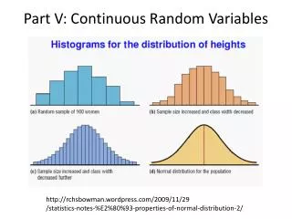
Normal Distribution N(μ,σ2) Normal Distribution (Gaussian Distribution) with parameters μ and σ2 > 0 if its probability density function ƒ is given by for -∞ < x < ∞ *Where μ = mean and σ2 = standard deviation* Distribution function is given by: for -∞ < a < ∞ However, since ƒ does not have an antiderivative there is no explicit expression for Ƒ. Therefore standard normal distribution where N(0,1) is given as follows, and the distribution function is obtained similarly denoted by capital phi. for -∞ < x < ∞
Quantiles Portions of the whole which increase from left to right, meaning the 0th percentile is on the left hand side and the 100th percentile is on the right side. Let X be a continuous random variable and let p be a number between 0 and 1. The pth quantile or 100pth percentile of the distribution of X is the smallest number qp such that Ƒ(qp) = P(X ≤ qp) = p The median is the 50th percentile

